Contents
Introduction
Ruby is a graphical cross tabulator and data analysis program.
Functionality includes:
Data import from all commonly used data collection tools, for both ad hoc single import jobs and complex tracking jobs
Data cleaning and validation (Note that cleaning is usually done in the collection application, but Ruby has the tools if needed)
Variable constructions and automated verbatim coding
Report generation
Analysis
Export (including two-way communications with MSOffice programs)
Automation (a rich set of scripting/programming commands provided in libraries)
Job configuration for on-line display in Ruby Laser
Ruby GUI Help covers how to use the Graphical User Interface and the underlying concepts of data organisation, manipulation and tabulation.
This document was last updated on 14/01/2025.
GUI Overview
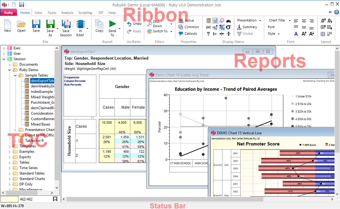
The top level Graphical User Interface elements are the Ribbon, Table of Contents (TOC), Report Display Pane, and Status Bar.
Splash Screen
The splash screen at start-up time shows release and licence information.
A subset of this form can also be opened with the Help About button
 on the Ribbon. Use this to directly access your Ruby Release version number.
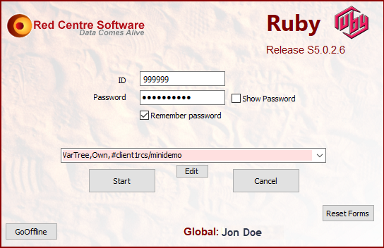
If you are running Ruby for the first time on this machine, or if the licence has changed (a new user on an existing Ruby installation)
Enter your licence ID and Password
Select a job (or -none-)
Click Start
On subsequent runs the splash screen dropdown lists the most recently accessed jobs.
Select --none-- to open with no job. This is useful if the last job has been so damaged that Ruby fails to proceed.
If you do not have multiple previous jobs the job list does not appear.
Edit: The displayed job list is editable via the Edit button directly under the job list.
Reset Forms:
 is the same as
  (see Forms Group), except that the reset can be done before displaying any forms. This addresses issues which can arise when moving from multiple to a single monitor, and the main Ruby form was last displayed on a monitor no longer connected. The default single-monitor form positions are restored.
Go Offline: Set your licence as local for up to a month. See below for details.
Internet Connection
You must have an internet connection to run Ruby in normal circumstances.
There are two ways to run Ruby without a connection:
1. Go Offline
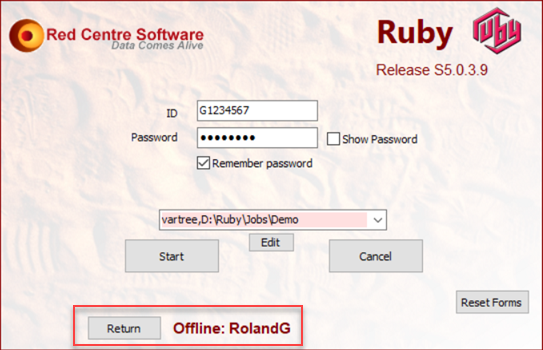
If you are travelling and expect to have difficulty getting reliable internet then you can prepare for this with the GoOffline button. You must have a connection to do this.
This stores your licence information on your machine and uses that until you return the licence. The GoOffline button is then replaced by a Return button.
This will last a month - then you will need to find a connection again.
2. Emergency
If you are caught without a connection, you will get this message:
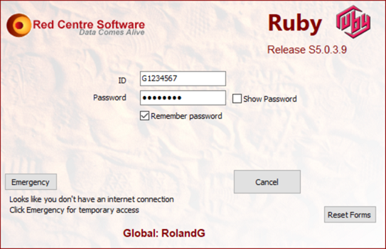
Click on the Emergency button to open this form:
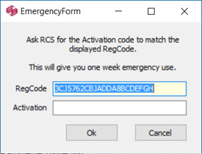
Copy/paste the RegCode to an email and send to RCS. An Activation code will be sent to you as soon as possible. Enter that code to continue for a week.
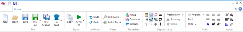
Ribbon
Related commands are organised on the Ribbon into the Application Menu, Tabs and Groups. The Ribbon also contains a quick access toolbar and system buttons.
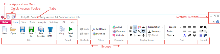
Ruby Application Menu
Home Tab
View Tab
Tools Tab
Analysis Tab
Scripting Tab
DP Tab
Help Tab
Quick Access Toolbar and System Buttons
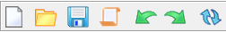
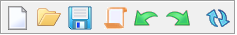
Quick Access Toolbar
Because these controls are so frequently used, they are duplicated here so that they are accessible whenever the Ribbon is showing, regardless of which tab is open.

 See Home Tab | File Group
System Buttons
 Minimise Ruby
 Maximise Ruby
 Close Ruby. You are prompted to save unsaved sessions and/or reports.
 Hide Ribbon
 Show Ribbon Help About. Opens the Ruby splash screen which shows the version number and your user name.
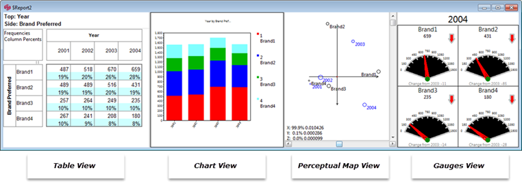
Report Display Pane
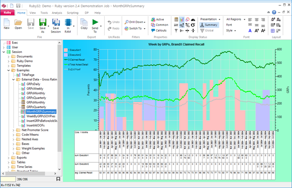
The Report Display Pane shows tabulated data. Four different views of the same data are available: tables, charts, perceptual maps, and gauges. Any or all of the views can be displayed in any order in the same window.
While usually you will have just one view active, it can be convenient, for example while looking at a chart or map, to also see the underlying table data.
On saving, the left most view is saved.
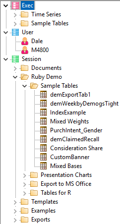
TOC
The Table of Contents (TOC) is for keeping track of tables, charts and other job-related files. The TOC looks similar to the standard Windows Explorer tree and is an organised collection of all the reports and associated other documents for the job.
The three main user types (Exec, User, Session) are designed to make it easy to organise reports into presentations and to make them available to the three different types of users.
The Session node in the Table of Contents is where users save and access reports and other documents for their own use.
The User and Exec sections are for shared LAN or Cloud jobs. These provide a way for users to post reports for each other and to finalise a set of reports for executives or for client reporting.
The Exec section is also used as a storage location for read-only reports, visible to all users of Ruby Laser (for on-line reports).
When working on a LAN or online/Cloud job all three sections are always visible.
When working on a local drive, you can hide or show the Exec and User sections from the Preferences form.
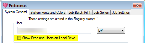
If you are not connected to a network, the Exec and User sections will refer to your local drive, and can be used to make copies or backups of the reports in Session.
In general, most work is done in the Session section, which defaults to show files on your local drive. To upload some reports to the LAN or for an online job, simply drag them from Session to User or Exec. To download a copy of reports in User or Exec, simply drag them down to Session.
For online jobs, Session reports can optionally be saved to the cloud.
Each user has a private session. This is useful if you want to guarantee off-site backup for everything.
Viewing Reports and Documents
Double-click on any report in the TOC to view it. Reports display in the report display pane on the right side of the screen.
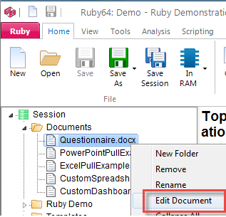
All Microsoft files, PDFs and other file types will open in their native program outside Ruby. This enables you to store all files and documents related to the job in a single place, thereby reducing the opportunities for losing documents over the life of the job.
To open a document for editing either double-click the file name or use the right-mouse context menu and select Edit Document.
Session
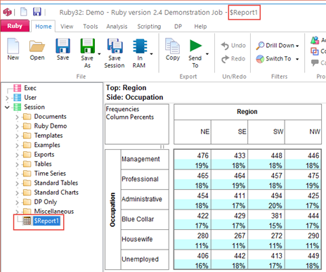
Every time you create a new report (table or chart) it appears in the Session section after the currently selected report or as a child of the selected folder. The new report will have a default temporary name, like $Report1, that will be removed if you decline to save it later under a permanent name.
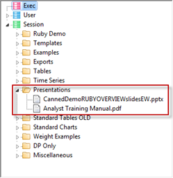
Any other type of file appears as a document node, such as the PowerPoint and PDF files shown here in the Presentations folder:
Session Context Menu
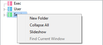
A right-mouse click on any item in the Session branch of the TOC displays the context menu.
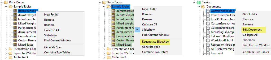
If a slideshow is active, then the Regenerate item appears.
New Folder: create a new folder
Remove: remove a node and all child nodes - you can also remove with the [Delete] key
Edit Name: used to rename a node - you can also rename in situ using the standard Windows slow second click on the report name
Edit Document: (appears over a non-chart/table node, such as a shortcut to a text file, Word doc or even an executable file) - this opens the document in its natural editor as if you had double-clicked on it in Windows Explorer
Collapse All: close all folders
Slideshow: starts a Slideshow to display the reports in the current folder in a single window
Find Current Window: highlights the node for the currently active report window
Regenerate Slideshow: Regenerate all slideshow reports using a different top/side/filter/weight. See Regen SlideShow form.
Generate Spec: generate script syntax that specifies the report under the mouse or the active slideshow in the TOC. See here for a detailed description.
Combine Two Tables: Add, subtract, multiply or divide two tables
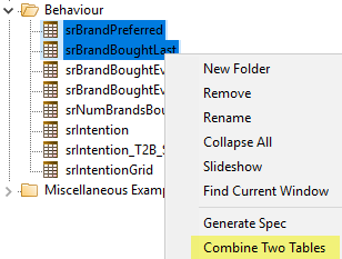
The operands are in the selection order. Use Control/click to select.
A right-mouse click on the Session node itself displays a limited number of options.
You can rearrange items under the Session node using drag and drop or the [Ctrl]-Arrow keys, as in most tree views in Ruby. (See TOC Tree Exercises.)
The arrangement in the Session section (unlike the User and Exec sections) does not reflect the directory structure on your disk. All reports are stored under the ReportsSession directory somewhere.
You can move items anywhere in the Session branch of the tree and that will not change where the files are stored on disk.
You can save reports in subdirectories under ReportsSession and that will not be reflected in the tree.
Regenerate Slideshow form
Regenerate the currently selected slideshow with replacements for any of the top axis, side axis, table filter, weight and case filter. A new filter can be appended to any existing report filters. A blank or disabled field for Axes, Table Filter, Weight or Case Filter means to keep the original.
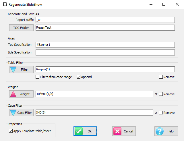
The above settings will:
generate new names from the originals with _w suffix
store the new reports in the TOC folder RegenTest
replace the Top axis with axis Banner1
append Region(1) to any existing filters or make it the filter if no existing filter
weight to 10 multiplied by codes 1 to 5 of BBL, 0 otherwise
case filter to those who passed the Industry screener, and
apply the current table and/or chart template.
The side specification, because empty, will remain as per the original reports.
The axes, filters and weight are entered using GenTab syntax.
The Remove check boxes will remove the existing filter/weight/casefilter. These are needed because an empty field means no change to the original. If a Remove is checked, the rest of the group is disabled, and any current entries are ignored. Remove always removes the original table specification part completely.
Report suffix: A small string to append to the existing report names, eg if filtering to Males, then _male would be a sensible choice.
TOC Folder: The Table of Contents folder for the new reports
Top Specification: A replacement top axis in GenTab syntax
Side Specification: A replacement side axis in GenTab syntax
Filter: A filter in GenTab syntax to either replace the original entirely, or, if Append is checked, to append to any existing filters
Filters from Code Range: Run the regeneration once for each code in the filter range, for example, using Gender(*)
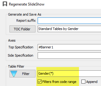
The regeneration is
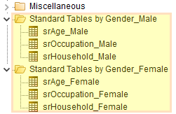
Note that a report suffix is optional because the filter code labels are also used to generate the names.
Weight: A replacement weight in GenTab syntax
Case Filter: A replacement case filter in GenTab syntax. A case filter works by simple lookup, so the filter must be only a value range of a single-response variable
Apply Template: Use the currently designated template table for regenerated tables, and the currently designated template chart for regenerated charts
For GenTab syntax details, see the API help topic Appendix 5: GenTab Syntax for Axes Specifications.
This is a powerful facility, so be careful. Changing all the specification parts simultaneously will generate the same table repeatedly, once for each original slideshow item. Typical usage is changing just the top axis (for a different banner), running weighted versus unweighted, demographic splits, different periods defined by case filters, etc. But sometimes the banner is on the side axis, so all possibilities must be accounted for.
Generate Spec
Ruby can automate the generation of reports via scripting. This is covered in detail in the RubyAPI.chm, which can be accessed from the Help tab of the Ribbon.
The right-mouse context menu item, Generate Spec, can be applied to a single report in the TOC, or to all the reports in an active Slideshow.
The generated code appears in a text file that can be saved, thus providing a means to recreate the report at a later time.
Scripts can be generated as:
VBS/VBA
VB.NET
JScript
C#/CSX
SPX
VBS (VB Script) and VBA (Visual Basic for Applications) are essentially the same as the MS Office macro language. Use the Ruby script editor AutoEdit or any MS Office macro editor to execute. Excel is a common choice.
VB.Net can be executed in Microsoft's Visual Studio or VS Code. It is a fully professional programing language.
JScript is Microsoft's simplified Java. It is closer to the hardware than VBS/VBA, and the syntax is fussier than the VB family. Use AutoEdit to execute.
C# can be executed in Visual Studio or VS Code, and by various command line tools. It is a fully professional programing language.
CSX is the script-friendly simplified version of C#. CSX is the default scripting language for the Carbon DLLs.
SPX (for table specs) is a proprietary format for use by Diamond (part of the Carbon suite). Its syntax is as minimal as possible. See the Diamond documentation for details.
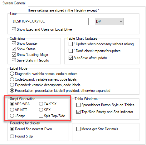
The script type is selected on the System General tab of the Preferences form:
Regardless of the report type selected for Generate Spec (Table, Chart, Perceptual Map, KPI Gauge), the code created will specify just the underlying table.
The generated script is not turn-key. You must provide the calling framework and declare required variables.
For this table
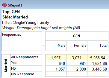
the generated script in each language is:
VBS/VBA
name='$Report1'
top='GEN(cwf;1/2;tot%)'
side='Married(cwf;1/2;nes%No Response)'
filt='Household(1/3)'
wght='WghtAgeGenRegCell()'
Set rep=rub.GenTab(name,top,side,filt,wght)
VB.NET (same as VBS/VBA, but does not need Set for assigning the report object reference)
name='$Report1'
top='GEN(1/2;tot%)'
side='Married(cwfAll Respondents;1/2;nes%No Response)'
filt='Household(1/3)'
wght='WghtAgeGenRegCell()'
rep=rub.GenTab(name,top,side,filt,wght)
JScript (since is the escape character, needs \...\ for label overrides, and lines must end with ;)
name='$Report1';
top='GEN(1/2;tot%)';
side='Married(cwf\All Respondents\;1/2;nes%\No Response\)';
filt='Household(1/3)';
wght='WghtAgeGenRegCell()';
rep=rub.GenTab(name,top,side,filt,wght);
C#/CSX (same as JScript, except that a leading @ means \ is not required for override labels)
name='$Report1';
top='GEN(1/2;tot%)';
side=@'Married(cwfAll Respondents;1/2;nes%No Response)';
filt='Household(1/3)';
wght='WghtAgeGenRegCell()';
rep=rub.GenTab(name,top,side,filt,wght);
SPX (the internal and very simple table specification system for Diamond)
name=$Report1
top=GEN(1/2;tot%)
side=Married(cwfAll Respondents;1/2;nes%No Response)
filter=Household(1/3)
weight=WghtAgeGenRegCell()
Run
The SPX syntax does not require double quotes, declaring variables, or line terminators.
TOC Tree Views
Ruby generally uses Windows standards in its GUI, but has some special extensions designed to make typical tasks easier.
This particularly applies to trees.
Lists of data and documents are frequently presented as tree structures.
Folders can be created, renamed and deleted.
For a hands-on exercise, click here
Reports can be opened, removed, reopened under different items in the tree.
For a hands-on exercise, click here.
Trees can be manipulated by either ordinary drag/drop operations or by the [Ctrl]-Arrow keys, which offer some extra functionality.
Ruby trees commonly have a search field at the bottom that can operate in three different modes, Character, Word or Find.
Tree Hotspots
There are two hotspots in Ruby trees - one to minimise all folders and subfolders; one to open all folders and subfolders (Note that your node icons may be triangles

 or boxes
 depending on your Windows theme settings):
TOC Tree Exercises
The six exercises that follow provide hands-on activities to develop skills in manipulating Ruby trees.
Exercise 1. Create and Rename a Folder
Exercise 2. Open, Remove, Reopen Reports
Exercise 3. Using the Ctrl-arrow keys
Exercise 4. Mouse Drag & Drop
Exercise 5. Using Search Fields
Exercise 6. Collapse and Hold
1. Create and Rename a Folder
Right-click in the blank space under the last item in the tree and select New Folder
This makes a new folder at the bottom of the tree and selects it.
If you click the new folder before doing anything else you can rename it in situ. If the folder was not already selected, this would require two clicks: one to select, and one to enter Edit mode.
You can also use the right-mouse menu item Rename to open an Edit dialog.
Using either a single click if selected, a slow double click if not, or the right mouse context menu item Edit Name, change the name to Test and press [Enter]
Continue to Exercise 2
2. Open, Remove, Reopen Reports
Select the Test folder just created in Ex 1.
 Select Open from the Home tab.
Select the file ATest.rpt and click OK (or double-click the file name)
A table window opens and a new entry appears in the TOC under the Test folder (middle picture above).
Reports added to the TOC appear under the currently selected item, in this case the folder Test.
To place the report elsewhere, select a different branch first.
To see this in action:
First remove the ATest item using the right-mouse item Remove or just press the [Delete] key
Now click on the Session folder further up to select it
Load ATest again (Home Open
 ) - ATest opens at the bottom of the tree
Hold the Ctrl key and press the right arrow key
This moves the selected item one level deeper so it is now a child of the Test folder.
[Ctrl][Left] arrow brings it back - but do not do that yet.
It is necessary to click on the ATest item before the [Ctrl] arrows work because focus had shifted to the table window.
3. Using the Ctrl-arrow keys
To move entire folders
Select the Test folder with a single click
Press [Ctrl][Up] arrow a few times to bring Test underneath Exports
Notice the entire folder travels as a single unit.
Now press [Ctrl][Right] again
This moves the Test folder to under the Exports folder as its last child.
You can use the [Ctrl] arrows to do almost any rearranging of the tree you wish.
You can even do unusual things like making one table a child of another table or make folders subordinate to tables and charts.
You may choose to do this to show a set of filtered charts under an unfiltered parent, or a set of different zooms of the same parent, or any other set of appropriate variations.
Care should be taken to ensure that your TOC arrangements make sense to other users of the job.
4. Mouse Drag & Drop
You can achieve the same result using the mouse instead.
Open the Test folder and the Exports/Charts folder by clicking the [+] or double-clicking the node
Click on the ATest item and without releasing the mouse button drag the item up and drop it on the Area item
Notice that ATest lands above Area.
Now drag ATest down and drop it on the SinglePie item
Notice it lands after SinglePie this time. When you drop an item it lands before or after depending on which direction you came from.
Drag again and drop on the Test folder
It does not matter which direction you come from when dropping on a folder - the dragged item always becomes the last child of the folder.
To return the TOC to its original state
Remove the Test folder by clicking on it and pressing [Delete], or by using the right-mouse menu item Remove. Answer Yes to the confirmation prompt.
Close up the Exports folder by clicking on the [-] box or by double-clicking the folder
5. Using Search Fields
At the bottom left of the TOC is a search field.
Type gen in the search field
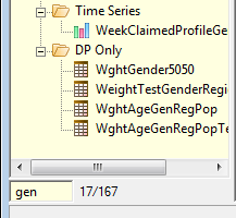
This filters the display to only those items with the sub-string gen somewhere in them, while retaining their parent branches.
The background of the display turns yellow to indicate the list is filtered.
The count beside the search field indicates how many items are visible out of how many altogether (here, 17/167). (Your own installation may show a different ratio of items.)
The search field operates in three ways: character by character, word within words, or next occurrence of a word.
There is a right-mouse menu on the field for changing the search mode:
A yellow background indicates Character mode
A green background indicates Word mode
A blue background indicates Find mode
In Character mode, the search is updated every time you press a key - including delete and backspace.
In Word mode a search is not initiated until you press [Enter].
On typing a word (or word fragment) and pressing [Enter], the list is filtered to only items containing that word somewhere.
Type in another word and press [Enter] again and the already filtered list is further filtered to those items also having the second word, and so on.
Right-click in the search field and change to Word mode
Type in gen and press [Enter] - you see everything containing gen and the search field is cleared ready for the next word
Type in week, press [Enter] and you see everything that contains both gen and week
Press [Enter] on an empty search field to return to the unfiltered state
Find mode jumps from one match to the next as you press [Enter].
Right-click in the search field and change to Find mode
Type in gen and press [Enter] - the highlight jumps to the first match and the search field is not cleared
Press [Enter] again and the highlight jumps to the next match - and so on, cycling back to the top to start again when there are no more below
The three search modes are very useful for navigating huge trees.
6. Collapse and Hold
You can close all open branches with the right-mouse item Collapse All or by clicking on the hotspot (see TOC Tree Views) at the top-left of the tree.
In Char and Word mode, if you backspace to an empty field all open branches except those for the highlighted item are collapsed.
Make sure the search field is in Char mode and type in gen
Click on the one chart under Time Series to make it the selected one
Now click back in the search field and back-space or delete the text
You will see lots of open branches as the search string is reduced but at the last backspace, when the field is empty, all branches except the one with your selected item are collapsed.
Table Window
This section covers mouse control over the various properties of table displays.
You can resize at many points, change font style and size, undo and redo commands, and there are several right mouse context popup menus.
There are also indicators for Top/side priority at intersections and row/column sorting.
For detailed help on Properties, see Properties Group.
Resizing
All table resizing is done from the top and side label areas. To resize body cells you change the label cells.
The diagram below shows the hotspots for resizing when the cursor changes to a standard resizer:
1. The line separating the row/column labels from the group labels can be moved to change how the internal space is shared between labels and groups. If there are several levels of grouping, the group space is shared equally between all levels. You can make the group columns all wider or narrower but you cannot specify different widths for different groups.
2. The line where the labels end can be moved to change the length of the label cells without affecting the group lines.
3. The width of label cells (height of side labels, width of top labels), and hence of the body cells can be changed by dragging the very first inside line.
4. You can change the label width indirectly by dragging the end lines of the label areas to change the overall space occupied by the labels.
5. The title area is initialised as just big enough to hold all titles and can be resized by dragging the divider.
 It is difficult to make the table unreadable by accident but it can be done. If this does happen you can always fix things clicking Undo on the Ribbon or by changing the property values directly on the Labels tab of the Table Properties form.
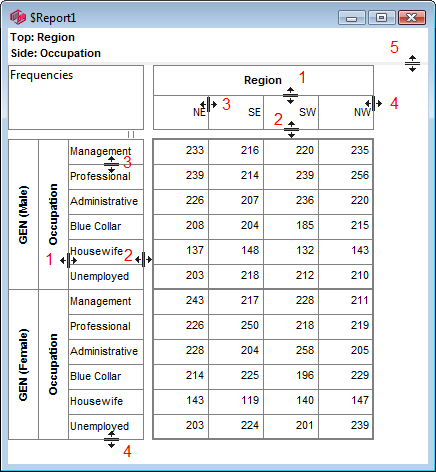
To resize everything uniformly up or down, use the controls in the Layout group on the Home tab of the Ribbon.
Fonts
For details see Font Group.
Undo, Redo on Tables

When there is something to undo, the Undo button on the Home tab of the Ribbon becomes active. Clicking on it undoes the last change, and clicking on the Redo button redoes the last Undo.
Undo/Redo applies to any resizing or drag actions with the mouse, and to Segment or Drill filters.
Right-mouse Menus
There are four different right mouse menus available on the Table display. The coloured areas show where each is accessed. Some of the items correspond to controls on the Ribbon.
1. The Titles menu
(shaded green), is for changing the Presentation Mode labelling.
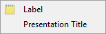
Label: Change the Presentation Mode text for each of the four items in the title - Top, Side, Filter, Weight/Modifiers.
Presentation Title: Provide a single piece of text to replace all four individual items.
2. The Labels menu
(shaded blue), available on the row and column labels area, allows functions for one particular row/column or one of the nested labels.
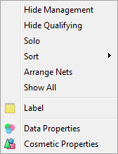
Hide: Hide this row or column from display.
The selected vector's label is dynamically shown as the first item, here 'Hide Management', where 'Management' is the label under the right-click.
To reveal the row/column again, select Show All.
Hide Qualifying: This toggles hiding or showing rows/columns that meet the settings in Properties Hide.
This is usually missing or zero data but could be relative to any reference number.
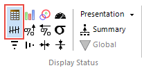
This corresponds to the toggle buttons on the Display Status group on the Home tab of the Ribbon:


Solo: Hide all other rows/columns but this one.
Sort: Rearrange the table so that values in this row/column are sorted. In the sub-menu you can choose to sort by column value, code or label (alphabetical).
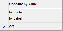
These settings are in Properties Sort. This also corresponds to the toggle buttons on the Display Status group on the Home tab of the Ribbon:

 .
.You can have some codes excluded from sorting. See Edit Variable form | Codes.
Arrange Nets: Nest and sort net expressions. See the Demo job reports SortedNets (arranged) and NetSort2 (before arranging).
Show All: Reveal all hidden rows/columns.
Label: Open the Label form for setting Presentation Mode text for this column.
Callouts: If the row or column is a simple code from a variable that has callouts they will appear as extra menu items with a callout icon
 . This has an attached sub-menu for playing any attachments:
Data Properties: Open the Common Properties form (the Vectors tab of Table Properties) with this row/column selected.
Cosmetic Properties: Open the Table Properties form at the Labels tab.
3. The Groups menu
(shaded yellow), is a subset of the vectors menu and contains table wide items.
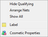
Hide Qualifying: Toggles hiding or showing rows/columns that meet the settings in Properties Hide. This is usually missing or zero data but could be relative to any reference number. The command corresponds to the toggle buttons on the Display Status group on the Home tab of the Ribbon

 .
.Arrange Nets: Sorts Nets with their subordinate variables indented underneath each net, arranged alphabetically.
Show All: Reveal all hidden rows/columns.
Label: Open the Label form for setting Presentation Mode text for this column.
Cosmetic Properties: Open the Table Properties form at the Labels tab.
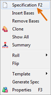
4. The Cells menu
(shaded pink), is the default that appears anywhere else on the window and contains table wide items.
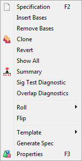
Specification: (Hot Key F2) Reopen the Table Specifications form populated with the specification for this table so that you can make changes and rerun it.
Insert Bases: Insert base rows and columns for each variable on both top and side axes.
Remove Bases: Remove all base rows and columns.
Clone: Create a new window with a duplicate of this table.
Revert: Reload the report from disk.
Show All: Reveal any hidden rows and columns.
Summary: Open the Summary Planner form.
Sig Test Diagnostics: This will appear if the table has significance testing turned on and saves a text file .sig in the the report's sub-directory with details of the calculations.
Overlap Diagnostics: This will appear if a table has the Overlap switch on a significance test and will save a text file .dmp in the the report's sub-directory with details of the calculations in a format similar to Quantum's tstat dump file.
Roll: Opens a sub-menu to change the roll for all rows/columns that allow rolling. There are a few presets and an item for entering a custom roll.
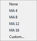
A variable can be excluded from rolling by right-mouse on the Edit Variable form. This is useful for external (non-survey/not sampled) data like sales turnover or advertising weight.
Flip: Swap rows and columns. The percentaging bases are also flipped, so column percents will become row percents, and vice versa.
Generate Spec: Generate script syntax that describes the report. This also appears on the Generate group on the Scripting tab. The syntax for the generation can be set on the Preferences form, System General tab, Script Generation group.
Template: This is a quick way to set the cosmetics of the current table as the template for all subsequent ones, or to apply the cosmetics of the current template table. If the job has a default template (shown in File | Preferences | Job Settings) then that can be overridden here.
Properties: (Hot Key F3) Open the Table Properties form at the last used tab.
Indicators
There are two indicators that can appear on the table in the gaps between the labels and cells. This determines which vector has priority at table intersections that are ambiguous - such as a top base intersecting with a side base.
Both of these indicators can be optionally hidden by turning off the Top/Side Priority Indicators switch on the System General tab of the Preferences form:
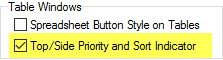
Chart Window
The Chart Window is very mouse-active to make it easy to work interactively with charts.
 The Undo/Redo buttons on the Home tab cover all mouse changes for recovering from mistakes.
When resizing a chart all graphics scale to keep, as near as possible, the same relative size and position. The only exception are *.ico graphics which cannot be resized at all.
Common fonts are generally well handled but the more exotic the greater the chance of minor mis-scaling. Font scaling is done by point size so you may see minor differences at different scales.
Areas in the Chart Window
There are seven types of active areas in a chart window:
Graph
Text
Pictures
Legends
Axes
Callouts
Summary
Except for the Axes areas (see below) general behaviour is conventional.
Drag: Left-click in an area to drag it to another position.
Stretch: The box outlines for Text, Pictures and Legends will stick after the first click so you can find them for resizing.
Click on the graph box to unstick the outline.
You can flip and invert pictures by stretching from a corner.
Double-click: will generally present the Chart Properties form opened to the most appropriate tab, the exceptions being Callouts and part of the Summary area.
Right-click: generally presents a context menu.
Where areas overlap the precedence is: Over Pictures, Text, Axes end points, Summary, Callouts, Legends, Axes, Graph, Under pictures.
General Context Menu
There is a general context menu (right-mouse) available everywhere except Axes, Legends and Callouts.
This is the same as the Table general context menu, but with some extra chart-specific items.
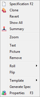
Zoom: enters Zoom mode.
Text: adds a new Text object to the chart.
Picture: adds a new Picture object to the chart.
Remove: removes the pointed-to object from the chart - this item only appears if right-clicking on a Text or Picture object.
Generate Spec: Generate script code for this chart.
Text
Text is multi-line. On resizing the selection box, the text will wrap around at word boundaries if possible or split the word if not. Sometimes you need to make the box taller or wider to reveal all the text (an ellipsis will show if this is necessary).
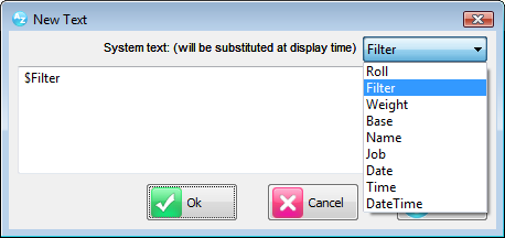
New Text Form
When you select Text from the menu a form appears with the text 'Default Text' in it. Replace as desired or select one of the System texts.
This is a multi-line field which recognises return characters.
If the text is exactly one of the special names like $Filter, $Roll (not followed by a [Return]) then it will be automatically generated on the chart.
$Name is the file name of the chart
$Title is the chart title
$Filter is the overall filter
$Weight is the overall weight
$Roll is the common roll applied to series
$Job is the job name
$Date is the current date
$Time is the current time
$DateTime is both date and time
$Base is the headcount (filtered but unweighted) of cases (see also Preferences|Job Settings for Base Count Tag)
The text generated for Filter, Base and Weight also depends on the Label Mode setting on the Display Status group of the Home tab.
Pictures
Pictures can be Under or Over. Under means that the picture will be drawn before the rest of the chart. Over means that the picture will be drawn after the rest of the chart.
Supported graphic types are .BMP, .JPG, .ICO, .WMF, .EMF. Not all graphic types can be transparent and .ICO files do not scale. Transparency and scalability are properties of the graphic type, and have nothing to do with Ruby.
When adding a picture to a chart, the file is copied into the job's Media directory if it is not already there.
Legends
Legends can be in three styles: Linear, Nested or Tree. See Legends tab in the Chart Properties section for more information.
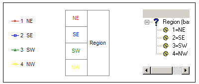
The Linear style is a conventional list.
The labels will word wrap at the invisible right boundary and you can see more or less text by resizing the bounding box.
The Nested version appears very much like the side labels on a table (although they may actually be the top labels depending on the XView setting toggled by the Flip menu item).
The leaf nodes are coloured for the series they represent.
You can resize the rows and columns by dragging.
The Tree style shows the variable(s) exactly as in the specification form.
Both the Linear and Nested versions have nearly the same mouse responses.
A double-click anywhere opens the Properties form at the Legends tab.
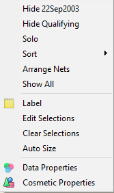
A right-click presents the Vectors menu.
As well as all the table items there are several others which are appropriate only for charts.
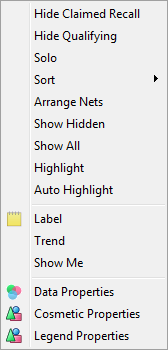
Highlight: draw this line series thicker and on top of other series.
Auto Highlight: toggles Auto Highlight mode (Linear style only). When this is checked you can highlight a series simply by holding the left-click on the legend for half a second. This is a convenient way to quickly highlight many series in succession. Select the menu item again to turn it off.
Trend: toggles showing the trend for a series.
Show Me: opens a form to place selections on the category axis at all points where the series meets a given criterion such as not zero, greater than 50 etc.
Legend Properties: opens the Chart Properties form at the Legends tab.
Any other menu items appearing after this are callout menus for the series, the same as appear on variable trees and table labels.
Chart Axes
Double clicking is different inside and outside the graph box.
There is a thin gap in the middle of the area so the graph box edge can be reached for dragging.
The Category axis uses the Vector menu from the Table form with a couple of extra items.
Areas
Single click:
End points - arrow cursor while dragging start/end values in or out
Inside/Outside - nothing
Gap - resize cursor, drag graph box edge
Double click:
Inside - arrow cursor while inside, can click-drag to highlight selection
Outside - properties form, Axes tab with this axis selected
Gap - properties form
Right-click:
Inside/Outside - Vector popup menu with Axis extras
Gap - Main form popup
End Points - click and drag
Left-click in the patch around the start or end point of an axis outside the graph box.
While holding the mouse button down you can drag the start or end in either direction to a new value (shown as text that floats with the cursor).
When you release the button the chart is redrawn with the new setting.
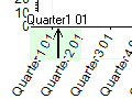
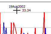
Category Axis Cursor - double click inside
Double-click in the Axis area just inside the graph box and the cursor switches to an Axis Cursor. This cursor remains until you move the mouse outside the graph box.
Text showing the value on the axis floats with the cursor so you can use it as a quick way of reading the label at any point on the graph. While in this mode you can also drag out selections on the axis for piece-wise trend lines and for summary tables.
Properties - double click outside
A double-click on the axis labels opens the Chart Properties form at the Axes tab with the axis selected.
Axis Menus
A right-click nearly anywhere in the Axis area presents the appropriate Axis menu.
Do not go too close to the graph box line, on which the axis is drawn, because there is a small gap in the Axis area, so the mouse can 'see through' to the Graph box lines for resizing.
A Category axis includes the table Label popup menu items (and callouts if available) with three extra items for axes.
For a Value axis you only see the items Autosize and Cosmetic Properties.
Edit Selections: opens the Edit Axis Selections form for precision editing of selections.
Clear Selections: clears any selections on the axis.
AutoSize: Shows the state of the AutoSize switch for the axis and allows toggling it.
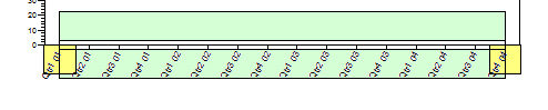
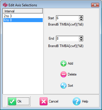
Edit Axis Selections form
For a date axis, the Edit Axis Selections form will appear with the selected intervals identified by start/end dates.
For a non-date axis the intervals are identified by start/end indices.
You can click on an interval to see its details, edit start/end points with the thumbwheels, add new intervals, delete intervals and sort them.
On clicking OK the intervals are sorted and a check is made for overlaps. If an overlap is found the form will not close and you will need to fix it first. Other than that the form is very forgiving - for example it will invert intervals that have start/end around the wrong way.
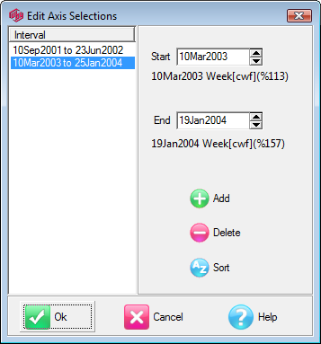
Note that a date axis is a single variable in Modified Julian Date format
Nested Axes
Axes can be nested just like Legends so they appear as they would on the underlying table.
In this style you can do most of the resizing available on tables except that the label box width (or height for a vertical axis) is determined by the extent of the axis and cannot be resized directly.
You can get the callout menu just as on the table. Callouts can also be added to the chart with the Chart/Callouts menu item or Toolbar button.
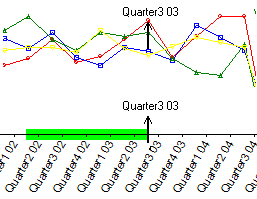
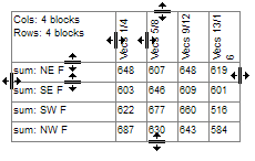
Summary Table
This table can be resized at any of the points indicated.
Double-clicking on the cells opens the Summary Planner form for changing the calculations shown in the summary.
Double-clicking on the labels or top corner opens the Chart Properties form at the Summary tab for changing cosmetic features of the summary table.
Adding Callouts
A callout comprises at least some short text, and optionally long text and file attachments. Callouts can be attached to any code of any variable. If the code is a date of a period variable, then callouts can be used to keep a record of all events which may affect question responses.
You can add callouts to the chart from the Chart Callouts form, on the Properties group of the Home tab.
Callouts appear as text boxes - multiline and stretchable. You can drag them anywhere, even outside the graph box.
When changing the axes, callouts move along with the point to which they are attached.
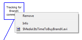
Double-clicking does nothing but right-clicking presents a context menu.
Remove: removes this callout from the chart.
Info: shows a longer description of the callout if available.
Files: other items will be file attachments that can be 'played' as if they were double-clicked in Explorer.
See the Concepts Callouts topic for more information.
Zoom mode
Selecting Zoom from the general menu changes to the Zoom cursor.
This will remain until you move the mouse outside the graph box.
The values of the X1 and Y1 axis float with the cursor so it is a convenient way to quickly read the coordinates of any point on the graph.
To zoom in on a part of the graph, left-click and drag out a rectangle.
On releasing the button the chart is redrawn with new axis values to match the zoom rectangle.
Use Undo on the Home tab to unzoom.Undo, Redo on Charts
When there is something to undo, the Undo button on the Home tab of the Ribbon becomes active. Clicking on it undoes the last change, and clicking on the Redo button redoes the last Undo.
These items register as something that can be undone:
ZOOM: dragging out a zoom rectangle.
GRAPH: any mouse shift or stretch of the graph box.
LEGEND: any mouse shift or stretch of the legends box.
AXIS: mouse drag of end points.
TEXT: any mouse shift or stretch of a text box.
PICTURE: any mouse shift or stretch of a picture box.
SUMMARY: any mouse shift or stretch of the summary report.
SELECTIONS: any changes to axis selections including via Edit Selections.
DRILL FILTERS: successive filters (including any segment filters) can be undone and redone.
SEGMENT FILTERS: successive filters (including any drill filters) can be undone and redone.
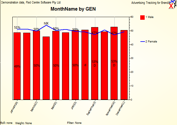
Data Labels and Significance
Significance results will appear on charts similar to the table display.
You can also elect to show Data Labels for each point.

Tests that display as changes to font colours on the table appear as exclamation points on charts.
Values can be set to show only on Major tick marks. See Series tab under the heading Data Labels / Major Labels.
Perceptual Maps
Correspondence Analysis
Ruby uses the standard correspondence analysis algorithm (cf SPSS, R, etc) to turn case data tables into perceptual maps.
“Correspondence Analysis provides tools for analysing the associations between rows and columns of a contingency table. The main idea of correspondence analysis is to develop simple indices that will show the relationship between the row and column categories.
These indices will tell us simultaneously which column categories have more weight in a row category and vice-versa.”
(Hardle, W., & Simar, L. (2007) Applied Multivariate Statistical Analysis. Second Edition. Springer, Heidelberg)
The index used is related to the Chi Square statistic.
Cells in the table are compared to their expected values and a new table formed from the chi square component of each cell.
This table is decomposed and the first few resulting eigen vectors for the rows and columns represent the dimensions in which the variation is greatest.
The first three dimensions are used to make a 3D plot of the categories.
Points that are heading in the same direction indicate categories that have an influence on each other.
To prevent maps from being too cluttered only the first 50 rows and 50 columns are passed to the map by default.
If you need more, the default is set at Max Map Points on the Job Settings tab of the Preferences form.
For more information, see:
Making a Perceptual Map
Perceptual Map Context Menu
See also:
Perceptual Map Properties
Making a Perceptual Map
The following exercise indicates how to show a table as a perceptual map.
 Start a new table in the Demo job
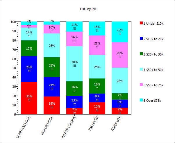
From the Demographics folder drag EDU to the top and INC to the side
Remove the No Answer code from EDU
 Click Run
Display as frequencies only
 Click the Show Map button in the Display Status Group on the Home tab of the Ribbon:
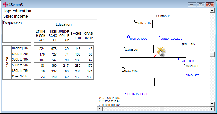
The map window appears showing the result of standard correspondence analysis of the table. As expected high income seems to be associated with high education.
The row and column vectors all appear as points on a two dimensional plane. Click anywhere on the plane to rotate the third dimension into view. This is often useful to confirm that an apparent association is not an artifact of perspective - a distant and close point appearing to overlap. It can also be useful to separate labels a little when they obscure each other. The scroll bars control this rotation as well.
Any table can be presented as a Perceptual Map but only the first 50 rows and the first 50 columns will be used. This limit prevents committing to an overly large map that would take time to calculate and not hold any usable information.
If you do need more than 50, the limit can be changed at Preferences Job Settings.
Perceptual Map Context Menu
This menu will appear when you right-click on a Perceptual Map report.
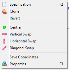
The first three items are identical to the table/chart main context menu.
Centre: return the display to no rotation into the third dimension
Vertical Swap: flip the display top to bottom
Horizontal Swap: flip the display on the diagonal
Save Coordinates: save the coordinates and eigenvalues in a text file for importing into other analysis software
Properties: open the Perceptual Map Properties form
Gauges
 A report can be viewed as set of Gauges by clicking the Show Gauges button on the Display Status Group on the Home tab of the Ribbon.
The report below shows both the Gauges and the underlying table.
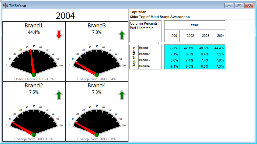
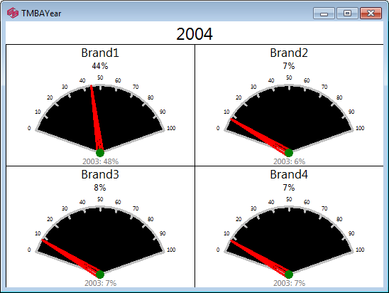
A Gauge shows the last column of the table in the gauge value displayed, and the second last column, underneath the gauge, either as a direct report (below) or as a difference (above).
These don't yet export yet and they are not exposed in the API.
Their main use is to allow preparation of a set of reports intended for online display in RCS's Laser product.
See also:
Gauge Properties
Status Bar
The Status Bar shows run-time information and flyover help:
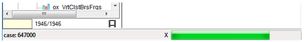
The progress bar can take a lot of CPU time to update on long table runs, so you may want to turn it off.
Status bar content can be set at Optimising on the System General tab of Preferences.
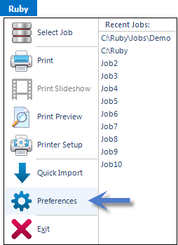
Ruby Application Menu
The Ruby Application menu is for job selection, hard copy printing, no fuss imports and setting various job-wide preferences. Items in this menu are comparatively infrequently used.
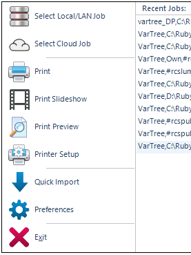
Select Local/LAN Job
Select Cloud Job
Print Slideshow
Print Preview
Printer Setup
Quick Import
Preferences
Exit
Select Local/LAN Job
Select a job stored on a local disk drive, or on your LAN (Local Area Network).
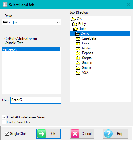
Drive: Select a local (usually C: or D:) drive or a network drived mapped to letter (typically N: or a letter higher than F)
Job Directory: Navigate to the job sub-directory - a Ruby job name is this sub-directory name, and the job is all files contained therein
Variable Tree: Select a variable tree - a variable tree exposes all or some variables, and a job can have as many *.vtr as you may require
User: Shows the name attached to your licence and will be the write-enabled folder under Users in the TOC
Load All Codeframes/Axes: Read and load all codeframes and axes details immediately. This is the default. If a job takes a long time to open (especially if a LAN job), then OFF will open the job almost instantly, and codeframes will load on demand (by double click or by using in a report specification).
Cache Variables: Load variables to RAM as required, and retain for possible reuse. This can improve LAN response times by avoiding redundant network traffic, but makes little difference for a local job in most circumstances
Single Click: Open folders with a single click rather than the traditional double-click
Ok: Open the job with the selected *.vtr
If a LAN job, then the form is
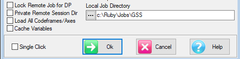
Lock Remote Job for DP: Lock out other users. This would be used by DP when doing job maintenance. Session reports are saved on the LAN, and are visible to anyone who is working directly on the LAN.
Private Remote Session Dir: Your Session reports are stored on the LAN. You would do this to have all your reports on the LAN for backup. Session reports are not visible to other users.
Local Job Directory: If reports are not being stored on the LAN, then you must specify a local sub-directory. These can be uploaded to your User folder or to the Exec section by drag-drop in the TOC.
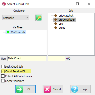
Select Cloud Job
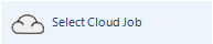
Cloud storage is organised by Customer.
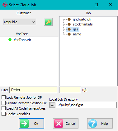
Customer: Select a Customer account from the top left drop down
Job: Select a Job from the list on the right
VarTree: Select a variable tree for this job
User: Shows the name attached to your licence and will be the write-enabled folder under Users in the TOC.
Lock Remote Job for DP: is the same function as for LAN jobs. The job is locked to other users while you carry out some DP functions.
Private Remote Session Dir: is the same function as for LAN jobs. It means your Session directory is in the Cloud under the Reports/CloudSession/username. You would do this to have all files on the Cloud for backup.
Local Job Directory: If Private Remote Session Dir is OFF then you need to identify a local job directory to store your Session reports. These can be uploaded to your User folder or to the Exec section by drag-drop in the TOC, in the same way as LAN jobs.
Load All Codeframes/Axes: A normal Vartree load from a cloud job just brings variable names and descriptions to save time. If OFF then codeframes are downloaded individually as required. If ON then all codeframes are loaded immediately on clicking OK. You would do this is you wanted all code labels available for searching, for instance.
Cache Variables: Download variables to RAM as required, and retain for possible reuse. This can improve response times by avoiding redundant data downloads. For a Cloud job, this would usually be ON. The only reason to leave OFF would be a need to keep as much free local RAM as possible, which is rarely an issue on 64 bit 16 gig or greater machines.

Ruby tables and charts will print directly to any printer.
Selecting the Print command from the Ruby Application Menu sends the report to your current printer without going via the conventional Print confirmation form. This is because all the settings such as Portrait/Landscape and page selections are done by Ruby, not Windows.
You can identify which printer will be used by first selecting Printer Setup.
You set print options in the report Properties|Page Setup tab, accessed by F3 or via the right-mouse menu on the report.
To batch print, use Print Slideshow.
To preview a table before printing, select Print Preview.
Print Slideshow

To batch print, first select a TOC branch as a Slide Show
 and then select the Ruby Application Menu command Print Slideshow. This opens the Print Slide Show form giving you an opportunity to check the batch settings before committing to the print. A summary of the settings is shown on the form:
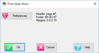
If not as required, then click the Preferences button to open the Job Batch Print tab of the Preferences form:
These settings will be applied to all reports except those which have the Override Batch Print settings switch ON at their individual Properties|Page Setup tab. This allows most reports to be, for example, portrait, with just a few set to print in landscape.
Print Preview

Opens the current table in the Print Preview window.
Print Preview applies to tables only as other report types print as they are displayed and do not have the same potential to take up multiple pages.
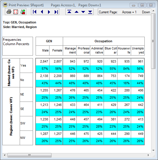
The caption shows how many pages will be produced by the printer. Navigate to any page using the arrow buttons at the top.
Open the Properties form
 to change things before printing.
Click the Shrink to Window button
 to see how the table will fit on the page.
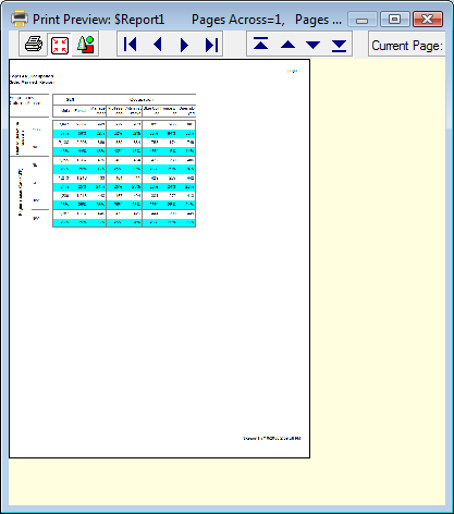
Printer Setup

Printer Setup opens the Windows Print Setup form for your currently selected printer.
Quick Import

A Quick Import is the fastest and simplest way to get case data into Ruby. The most common defaults for each import type are assumed. If the defaults are not appropriate, or if you need a more complex multi-file ID-linked (partial) import or a blended import, then use the Import form in the Tasks group on the DP Ribbon tab. The Quick Import form is most suitable for small ad hoc jobs.
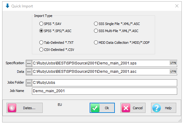
Import Type: the file format of the case data file(s) to be imported. See for details on the various supported formats.
Spec: The Specification or metadata file for multi-file imports (*.SPS, *.XML, *.MDD)
Data: The data file (*.ASC, *.DDF), or a single file if a single import file type (*.SAV, *.TXT, *.CSV)
Jobs Folder: The parent folder for the job sub-directory
Job Name: The name of the job
Dates: Set the date rules for the import as EU or USA, and the expected format for all-digit dates such as 20170209 = 9Feb17
OK: Run the import
Jobs Folder defaults to the current jobs folder (for the job you are currently in).
Job Name defaults to the Data file name stem.
The Jobs folder and the job name can be edited.
The Ruby import will exactly match the variable types in the original. Therefore, SAV and SPS/ASC will be fully normalised for multi-response, grids, loops, levels, SSS Single supports multi-response, but not grids, loops or levels, SSS Multifile supports levels, and IBM MDD/DDF supports all.
Preferences
The Preferences form contains general system settings (stored in the registry), and general job settings (stored in the file job.ini, located in each job's root directory).
Open either from the Ruby Menu or with [F4].
There are 5 tabs on the Preferences form:
System General
System Fonts and Colors
Job Batch Print
Job Series
Job Settings
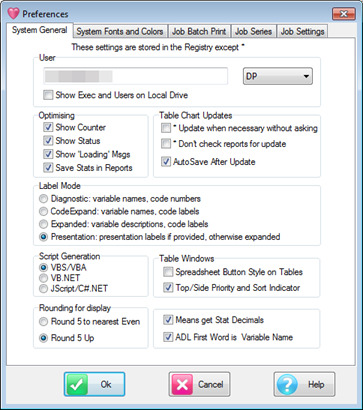
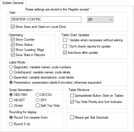
System General

System General settings control:
User Name and Type (DP, Analyst, Exec)
Optimising
Table/Chart Updates
Label Mode
Script Generation language
Table window display
Rounding method
other miscellaneous settings
User
If running locally, with DP full access, you can change your User name and access level.
The only result of a name change is a new user folder under the User section of the TOC.
User types are:
DP (full access to the job)
Analyst (access to all areas except DP Setup and Tasks)
Exec (Exec branch of TOC, view interactive reports, edit layout and cosmetics, apply drill and switch filters and export the results)
Note that an Exec user cannot create reports or save changes to existing reports.
Optimising
When running a large number of tables the counter and status messaging can become a significant part of the overall time. Either of these can be turned off.
You can turn off the Loading variable messages when a job loads.
If significance information is saved then reports load faster. If not saved, then the significance test will be rerun every time the report opens. For big reports, especially with Overlap tests, this can take a significant time. Note that scripted tests are always rerun when the table is loaded.
Table Chart Updates
When loading a table or chart Ruby checks if it has the latest data in it. If not, you are asked if you want to update it. Setting Update when necessary without asking to ON tells Ruby to update tables without interrupting with a prompt.
Setting the Don't check reports for update to ON stops Ruby from checking for updates. These switches are not saved in Job.INI.
AutoSave After Update is for when you get a prompt “Update report?” when opening a report. This means there is new data for the report. With this switch ON the report will be resaved after the update.
Label Mode
Labels on tables and charts can be diagnostic or descriptive in a variety of ways. See Label Modes for more information.
Script Generation
There are several ways to generate script syntax for existing tables (see Generate Spec for details). This setting determines what language syntax is used.
Table Windows
Spreadsheet Button Style: Changes the label style to solid buttons with light 3D effect.
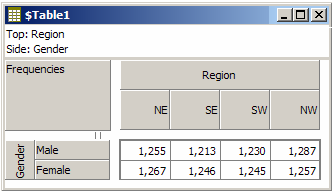
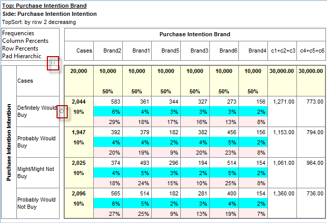
Top/Side Priority and Sort Indicator: Tables can show a small equal sign above the side labels or beside the top labels to indicate which way the addition is done to make the total for ambiguous cells (e.g. unweighted base row and weighted base column).
Tables can also show a small circle next to the current row or column sort key.
Rounding for display
When a number like 62.5 is rounded for display at zero decimal places should it be 62 or 63?
Microsoft applications like Excel always round such a number up to 63 so if you want things to look as they do in Excel you should choose 'Round 5 Up'.
In scientific and financial applications the rule is more commonly 'round to the nearest even' so that adding lots of numbers together is not biased upwards.
This setting does not affect calculations (Ruby always keeps numbers to 15 significant figures internally). It only matters when numbers are being prepared for display or clipping and the last digit is a 5, and when it is only that digit that is being rounded.
Means Get Stat Decimals:
The Table Properties has separate decimal settings for Frequencies, Percents, Statistics (green nodes) and Expressions (red and blue nodes).
Expressions like cmn#Region(1/5) or avg_BBL(1/10) [ie containing cmn or avg] can be treated as Statistics when determining decimals places.
System Fonts and Colors
The System Fonts and Colors tab provides control over colours, fonts and background graphics for Ruby's GUI.
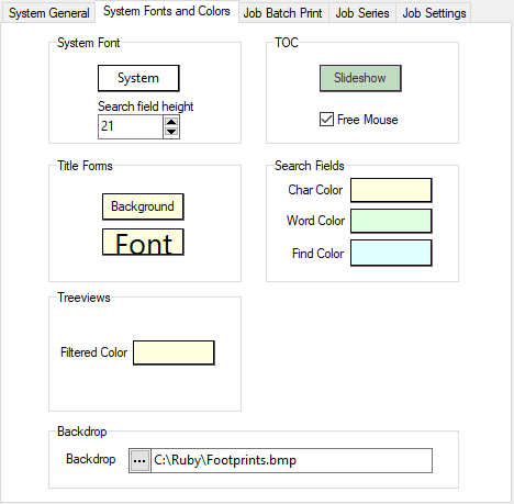
System Font
Ruby accommodates non-English scripts by allowing broad management of fonts.
All the trees, lists and edit fields use this System Font. If you need to show non-English (including Asian) characters you set the System Font to one with a suitable character set. When you first run Ruby this is set to your Windows Menu font so it is likely to be suitable immediately.
The Search Field Height enables adjustment of the size of the search box, to accommodate system font sizes too large to display in the default search box. This overcomes the problem of search fields appearing blank as a consequence of too large a system font.
TOC
You can change the highlight colour used in the TOC (Table of Contents) to indicate a slide show.
Free Mouse means that the slide show does not respond to mouse clicks so you are free to make mouse changes to tables and charts while in slide show mode.
With this switch OFF, a left-click will advance a slide and a right-click will go back to the previous one. In either case, the up/down arrow keys can be used for navigation.
Title Forms
When Ruby encounters a Folder node in the TOC during a slide show it shows a plain window with the folder's name in it.
You can set the colour of the window and the font to use.
Search Fields
The colour in the search field indicates which mode it is in. The defaults are pastel and can look washed out on some laptops. If you need stronger colours or prefer others, then change them here.
TreeViews
Set the background colour which indicates when a tree view is text-filtered.
Backdrop
You can have a picture on the main Ruby form behind all your reports. Most graphics file formats are supported.
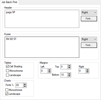
Job Batch Print
The Job Batch Print tab controls page settings and print output settings for tables and charts.
All settings except for chart font percentage reduction can be overridden per report at table and chart Properties Page Setup.
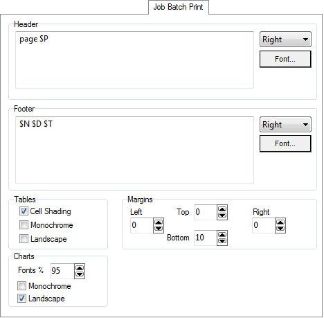
Header/Footer
This is the text that will appear as a header or footer on the printed page.
You can force white space by entering extra return characters and you can insert some dynamic information with substitution text.
$D is the date
$T is the time
$P is the page number (for batch printing)
$N is the file name
You can set alignment and font for these as well.
Margins
Printers vary somewhat. If more spare selvedge space is needed that can be set here.
Fonts
Printers also vary in how they treat fonts. Often fonts seem bigger on paper than on screen so you can make an adjustment here to reduce the size of all fonts.
Monochrome
This forces all fonts, lines and patterns to grey scale, and background and graph box to white. Pictures are left alone because most printers handle grey scaling automatically.
Landscape
Usually charts are printed one to a page in landscape mode.
When printing batches of charts, if two charts in a row are set to Portrait (Landscape off) they will both be printed on the one page, at half size.
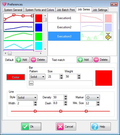
Job Series
The Job Series tab is for setting default chart cosmetics.
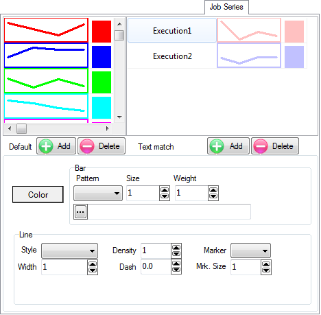
There are two sets of series cosmetics you can set up here.
Click
 to add a new one in either category,
  to remove one.
 The display shows a random line of four points which changes if you click it.
Default
The Default settings will be applied to any new series on a chart.
The display shows the system defaults for the first (e.g.) eight series.
The ninth series on a graph will collect setup number 1 etc. You are not limited to eight.
The cosmetic controls are the same as in the Chart Series tab.
Text Match
Sometimes you may want particular cosmetics on a code every time it appears on a chart.
You achieve this by picking some text that you know will always appear in the legend (whole words only) for that code and attach a cosmetic setup to it.
Job Settings
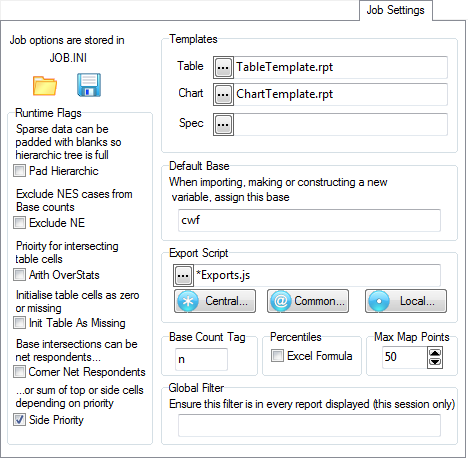
The Job Settings tab controls:
Templates - specifies the name of the default table template, chart template and the default specification.
Runtime flags
Default Base - most often set to cwf (Cases Weighted Filtered) but can be set here to any of the available base types
Your current export script - the standard script Exports.js can be modified and saved to a different name for custom or agency-specific behaviour
Base Count Tag - usually set to n, but can be any text required
Percentiles formula
Maximum Perceptual Map Points
Global Filter
Report and Specification Templates
You can identify a particular Table and Chart that will be used as default template for the job.
It is a good practice to include the word Template in the name of any template report.
You can always change the template dynamically to any other table and chart during a session using the report's right-mouse context menu.
You can also identify a default Specification. You would do this if you always used the same weight variable or preferred the Lock settings to be OFF by default.
This specification is loaded into the Specification form every time it opens or you click the New button on the form itself.
Default Base
Most jobs have a generally consistent way of basing most variables.
When a new variable is created, during import or by construction, it will be assigned the base (or base expression) stored here.
The most commonly used bases are cwf (Cases Weighted Filtered) and cuf (Cases Unweighted Filtered).
Export Script
The script to use for exporting reports to MSOffice. This is generally Exports.js but can be changed to a customised script.
Usually script customisation is performed by the programming team at Red Centre Software, but some organisations have the programming skills in-house.
Base Count Tag
You can have Base Counts appended to labels in tables, and charts have inbuilt $Base text - both are like “n=1000”.
The 'n' is the customisable Base Count Tag that can be set here.
Percentiles
Percentiles can be calculated a number of different ways.
The common method is: in N items the pth percentile is item p(N+1).
Excel uses a different formula: 1+p(N-1).
Ruby's default is the common formula and you can switch to match results from Excel.
Max Map Points
Perceptual Maps are too 'busy' if they have too many points. Set the maximum number of points to be displayed here.
Runtime Flags
See also Bases and Excluding Not Estabished.
These are the job defaults for table generation that can be changed for particular tables on the Specification form.
Pad Hierarchic: Hierarchic data is stored sparsely with the consequence that Not Established counts for empty nodes disappear, as if the table had been filtered to valid codes only.
Turning this flag ON guarantees that incomplete case hierarchies are padded with Not Established nodes.
Exclude Not Established (nes) from Bases: With this switch ON the bases (cwf, cwu etc.) are counts of valid cases only. See Bases and Excluding Not Established. Generally, this and the Pad Hierarchic switch should not both be ON.
Arith Over Stats: Cells on a table where the row and column are an arithmetic (red dot) and stat (green dot) normally show the stat result. This switch makes those intersection cells return the arithmetic result.
Initialise Table As: Tables can be initialised as all zeroes, or as all missing. The best choice for a given job depends on the data. Survey data would generally initialise tables as all zeroes. That way, an empty cell means no respondents met the cross tabulation criteria - i.e. zero respondents bought that brand or voted for that party.
In contrast, scientific data such as daily temperatures in meteorology often have zero has a legitimate source value, as in 0 degrees, which must be distinguished from days with no observations. In this case, the default for the job would be to initialise tables with the missing data token, displayed as *.
Corner Net Respondents: If you want the corner base cell in tables to always be Net Respondents set this switch ON. The Net value will then be used for percentaging bases and statistics that use the corner value (e.g. Single Cell).
Side Priority: Intersection cells for bases (including Corners described above) and arithmetic can be different depending on whether the top or side expression is followed.
Open/Save
All details are stored in JOB.INI automatically when you click OK but you might want to set up a few versions of JOB.INI for different circumstances.
You can save to any other name and load from any other name using the load and save buttons. (e.g. MYJOB.INI)
This doesn't set MYJOB.INI as the name of the default INI file. Instead it allows specific user choices to be manually loaded after Ruby is running.
Ruby only ever automatically recognises JOB.INI - loading it when the job is selected and saving it from this form.
Global Filter
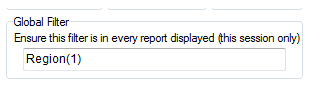
You can set a Global Filter in Preferences and turn it on/off on the Display Status group on the Home tab of the Ribbon:

This filters every table as it is generated, loaded or displayed.

The Global Filter appears in {curly braces} in the filter display, as shown in the table above.
Exit

Exit Ruby. You will be prompted to save unsaved sessions and/or reports.
Home Tab
The Home Tab of the Ribbon contains the most commonly used interactive items.
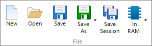
File Group:
Export Group:
Un/Redo Group:
Filters Group:
Properties Group:

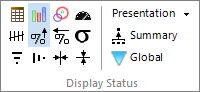
Display Status Group:
Font Group:
Layout Group:

File Group
New (Ctrl+N)
Opens the Specification form.
Open (Ctrl+O)
Opens a report (by default) but can also be used to open non-Ruby documents.
The opened file is added to the TOC. If the item is already present, you are prompted to add a duplicate. Sometimes duplicates are convenient, and so are not prevented.
Save (Ctrl+S)

Saves the current report - if the report is unsaved, you are prompted to provide a name for the report.
Unsaved reports are allocated a system name as $Report where index increases by 1 for each new unsaved report.
You cannot use $ in your own save-to names.
Save As (Ctrl+R)

Select Save As Ruby *.rpt to save the current report under a different name in Ruby report format (shortcut: Ctrl+R).
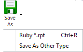
Select Save As Other Type to save the current report in one of the formats in the drop down list:
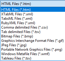
HTML: an HTML version of the table as drawn that will paste directly into Excel
XTabML: An industry standard format used by e-Tabs, QPSMR, and others, described at https://web.archive.org/web/20100226205809/http://www.xtabml.org/.
Use this format for imports to e-Tabs. For multiple reports, select as a slideshow on the TOC, then save under a suitable name. The multiple reports will be in a single file which e-Tabs will accept.
TabsML: An industry-standard format developed by e-Tabs, but now retired by e-Tabs in favor of XTabML
RubyXML: Ruby's own XML format (this is used mainly for internal purposes)
Comma delimited: Standard CSV file
Tab delimited: Similar to CSV with tabs
Bitmap: Standard BMP file
Graphics Interchange Format: Standard GIF file
Jpeg: Standard JPG file
Portable Network Graphics: Standard PNG file
Windows Metafile: Standard WMF file
Tableau: A text reorganisation of the table into a form suitable for Tableau imports. Contact RCS if you are interested in this facility.
/Docs is the default save directory, but you can choose to save elsewhere.
HTML and TabsML always use locale and never quote numbers. XTabML ignores locale. Internal files ignore locale: *.rpt and RubyXML always use dot for decimal, comma for thousands.
See also Export Group.
Save Session

Opens a Save dialog box to enable saving the current Session.toc under a new name.
Unsaved reports will raise a prompt.
In RAM (Ctrl+M)

Opens the In Memory form.
Shortcuts to the most common actions on the In Memory form are provided on the dropdown menu:
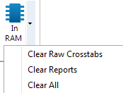
Ruby reports often comprise multiple raw crosstabs, where 'raw' means one top variable, one side variable, optionally filtered/weighted.
Clear Raw Crosstabs: When a report is specified, Ruby looks to see if the raw crosstabs are already in memory from previous specifications, and if so, uses them in preference to regenerating from disk.
Therefore, to force a full regeneration of all reports, clear the raw crosstabs first.
Clear Reports: Clears reports, but retains the raw crosstabs in case they are needed again.
Clear All: Clears all raw crosstabs and reports from RAM.
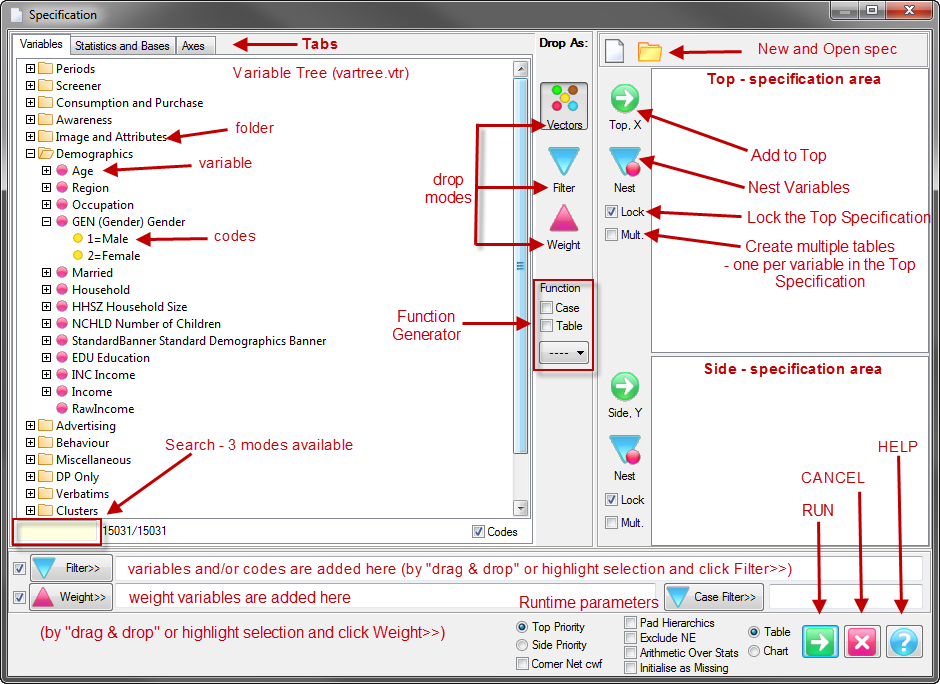
Specification Form
Report specification can be either by full variables, by individual codes of variables or by functions of either case data or vectors of tables. Any row or column (collectively, any vector) can be individually filtered and/or weighted, and any vector, filter or weight can be an expression. Statistics, Not Established, and any of the fourteen standard base types can also be selected as vectors for either the Top or Side axis. Bases for percentaging can be specified and inserted at any time, and percentaging itself can be turned on or off for each vector.
 (Ctrl+N) The New command on the Home tab of the Ribbon opens a new Specification Form. The top and side panels will be empty.
 F2 or selecting Specification from the right mouse menu on an existing report opens the Specification Form showing the specification for that report.
All Ruby users should aim to be completely familiar with the layout and operation of the Specification form as it is where all reports are created. If you are new to Ruby, Specifying a Simple Table is a good starting point. Much of the functionality of the Specification form relies on an understanding of the Ruby Algebra system. For details see Algebra in Concepts and Definitions.
If a specification is present, the top right toolbar shows as
The extra items are:
Save: Save the specification as a *.tbx file
Script: Generate the script for this specification
Undo: Undo the last specification change
Redo: Redo the last Undo
Flip: Invert the top and side axes. Note that this is different to flipping a report, which also inverts percentages, sort indices, charting direction, etc.
See also Local Tool Bar.
Local Tool Bar
The Specification form has a Local Tool bar located above the Top specification panel:
Use it to:
 Clear the current specification
 Open a saved specification
 Save the current specification
 Generate and show the script for the top, side, filter and weight components of the specification. For complicated specifications, it can often be easier to search/replace the script representation than to navigate and manipulate the trees. A typical usage would be to replace all instances of Q1 with Q2. On OK, the edited script is translated back into the trees and/or the weight and filter fields.
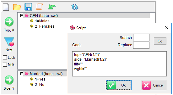
 Undo the last specification step
 Redo the last undo
 Invert the specification
Specifying a Simple Table
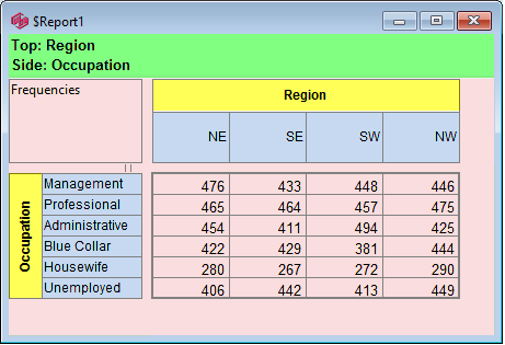
Follow these steps to specify a simple table comprising a single variable on the top and a single variable on the side.
Select New from the Home Tab of the Ribbon to open the Specification formLocate Region and Occupation in the Demographics folder
Drag Region to Top
Drag Occupation to Side
Click Run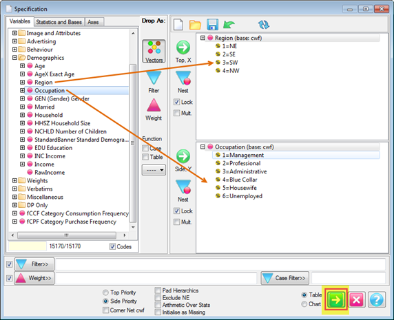
If the table is not showing frequencies only,
examine the Display Status settings on the Home Tab of the Ribbon and adjust the toggles so that only Display Table and Show Frequencies are toggled on:
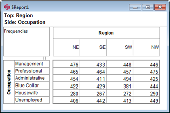
Open the Specification for the table you have just run by pressing F2 or selecting Specification from the right mouse menu on the table cells area:
Looking at Region in the Top specification tree, you can see that this variable has a base, cwf (abbreviation for Cases Weighted Filtered, the most common base type for survey data), and that each of NE, SE, SW and NW has a small % sign. Occupation is similar.
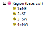
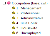

Together, these indicate that if the Column and Row percent buttons are toggled ON, then the frequencies will be percentaged on the indicated base.
Toggle ON the two percentage buttons (Col% and Row%) on the Ribbon:

 :
:Select Code from the Label Modes dropdown list:
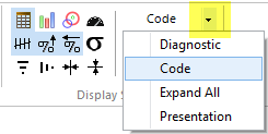
The resulting table is:
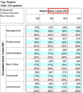
In any Display Mode other than Presentation, the Top and Side headings now report the base used for percentaging in parentheses - otherwise, you would have no idea where the percents came from. If the Display Mode is Presentation, then it is assumed that the meaning of the percentages is clear by the context.
Right-click in the Cells area and select Insert Bases
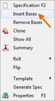
Note that the default state for bases is to display always as unpercentaged. This is so that it is easiest to make a table of column percents with the base values displayed as frequencies, the most common arrangement.
Toggle Frequencies and Row% OFF on the Ribbon:
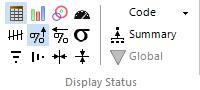
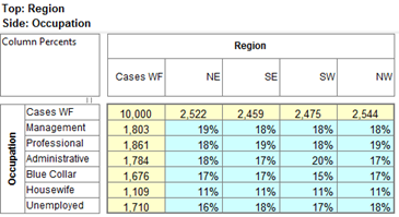
Note that the base is no longer reported in the top and side variable headings, because the table itself now tells you what the bases are. Only the coded cells have been percentaged. To see the base column counts as percentages of 10,000
Open the Specification for the table by pressing F2 or selecting Specification from the right mouse menu on the table cells area
Double-click on the Region cwf base node so that the small % sign appears
Repeat for the Occupation base node
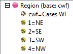
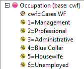
 Click Run
Toggle Row% ON too:
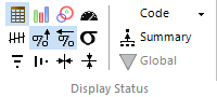
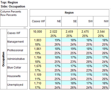
Looking at the top row, 100*2522/10000 = 25%, etc, and at the left column, 100*1803/10000=18%, etc.
Note that rather than show redundant 100% in the base vectors, Ruby instead shows just the base frequencies.
Close the table answering No to the Save prompt
Colour-coded Nodes
Colour-coding is used in Ruby to distinguish the different types of nodes, as shown below.
Note that double-clicking a node toggles between Unpercentaged and Percentaged (percentaged nodes contain a % sign in the node icon).
Dragging in the Specification Form
Many of the following exercises use drag/drop to get variables and codes into the various panels or edit fields. Often there are button-click alternatives and different users will develop preferred ways of working.

 Whenever you see 'drag the variable to the Top' you could equally 'highlight the variable and click the Top,X button. Similarly you can 'drag and drop' a variable to the Side or 'highlight the variable and click the Side,Y button.
There are some special behaviours for some drags:
Dragging a single folder to Top or Side is the same as dragging all the variables in the folder. (e.g. the Screener folder below)
Dragging a variable collects all codes and code arithmetic expressions.
You can multi-select codes and drag the selection. (e.g. codes 1, 2 and 3 for Age below)
You can drag items into the Filter/Weight fields or select and then click the Filter or Weight buttons at the bottom left of the form.
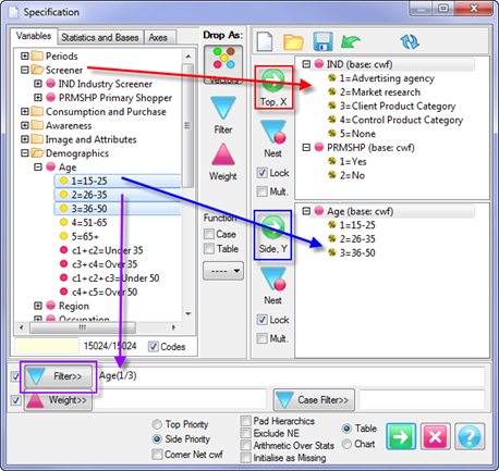
Adding Variables to Top and Side
There is no limit to the number of Top or Side variables.
Start a new tableDrag Married and Region to Top
Drag Gender and Occupation to Side
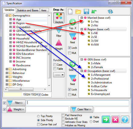 Click Run
 If your table looks different, adjust the Display Status toggles on the Ribbon to display frequencies only:
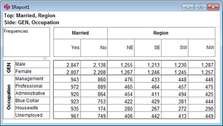
Bases and percentages can be applied as desired.
Multiple Tables - the Mult Switch
The table specification below contains four sub-tables - 2 top variables by 2 side variables.
You can have them appear as separate tables by using the 'Multiple' switches on the Specification form.
On this specification:
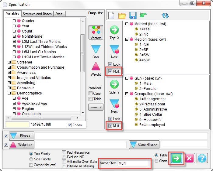
Turn ON both Multiple switches
This reveals another field where you provide a partial name for the set of tables that will be produced.
Type in a name stem (Multi)
Click Run
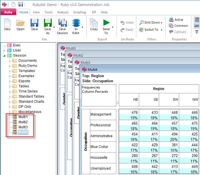
This produces four small tables instead of one big compound table.
The partial name, 'Multi' has a number postfix, incremented for each new table - Multi1, Multi2...
The Top and Side Multiple switches are independent so you can leave one compound and split the other - handy for compound banners against a number of individual variables. The split occurs at each root level node in the top/Side axis.
The tables are not saved yet so you will get “Save?” messages when you close them and if you decline the TOC entries will go away.
They are separate tables now, so you can't return to the compound specification, however you can save the specification (including the Multiple settings) from the Specification form itself. See Local Toolbar.
Close each of the Multi tables answering 'No' to the save prompt.
Axis Locks
The Axis locks are designed to allow intelligent updating of report specifications for jobs that are delivered in waves.
Consider the following specification of Week by BrandX and Brand1 only for BPRF, BBE and BBL.
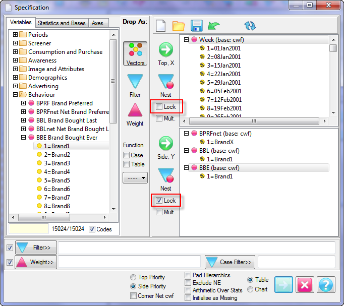
To allow the Week axis to extend, while preventing the Side axis from being extended when new data arrives, uncheck Lock Top and check Lock Side.
The intention is to have new weeks added automatically, but we do not want the system to assume that the three Brand measures have acquired extra codes too since the previous wave, because the point is to make a comparison between the three measures for the same brand 1 or its parent X.
The lock defaults to ON, on the assumption that it would generally be expected that, with no further action, a report specification will stay as specified.
Top/Side Context Menu
The right mouse context menu for a variable in the Top or Side panel is:
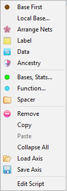
Base First: Make the first code under this code frame its base code
Local Base: Open the Select Base form to change the base for this code frame
Arrange Nets: Reorganise codes underneath nets
Label: Open the Label and Expression form to edit an expression or change a Presentation Label
Data: Open the Data form showing this variable's data
Ancestry: Open the Ancestry form showing this variable's construction ancestry (empty except for the codeframe if a source variable)
Bases, Stats: Open the Insert Statistics and Bases form to add any statistics or bases to all variables in this axis
Function: Open the Build Expression form to manually enter a function expression
Spacer: Insert a Spacer node in the axis (only between root nodes)
Remove: Remove the node under the mouse - same as [Delete] except you get a confirmation prompt
Copy: Copy the node under the mouse and its children for later pasting
Paste: Paste the most recently copied node
Collapse All: Collapse all open branches
Load Axis: Load a saved axis file (.axs in Specs folder)
Save Axis: Save as a .axs file in the Specs folder and add to the Axes tab
Edit Script: Generate and show the script for the top or side specification. For complicated specifications, it can often be easier to search/replace the script representation than to navigate and manipulate a tree. A typical usage would be to replace all instances of Q1 with Q2. On OK, the edited script is translated back into the tree representation.
Arrange Nets
Nets are recognised as sorting and arranging devices.
Codes are collected under the net and indented to show parentage. _net in the variable (orange dots) and net_var() functions in the spec (blue dots) are recognised as nets.
The sort is subnets within nets to any depth.
There are right-mouse menu items for organising nets on specifications or tables without sorting.
Here is a walk-through.
Open the table /Session/Examples/Other/NetSort2 (in Ruby Demo job version 5 only) or specify this table:
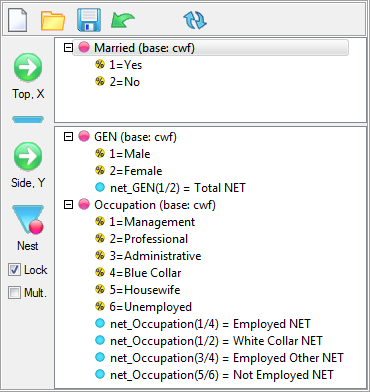
For details on how to create the nets, see Specify Nets on the Fly, Label and Expression Builder.
When run, the table appears as:
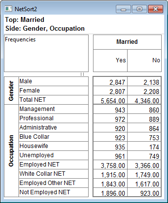
The side axis is in specification order.
The right-mouse context menu on the side labels is:
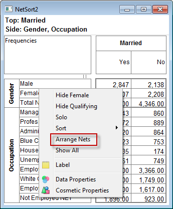
On selecting Arrange Nets, the table appears as:
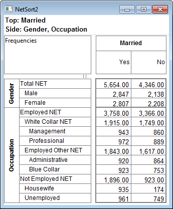
The Arrange Nets item in the context menu can be toggled on or off:
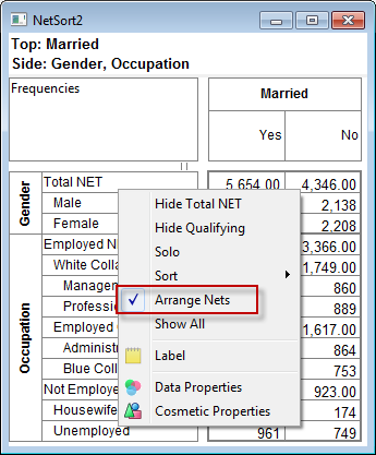
The same table in Diagnostic Display mode shows the net expressions.
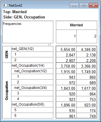
The Arrange Nets menu item is also available in the right-mouse context menu for the Top/Side axes in the Specification form:
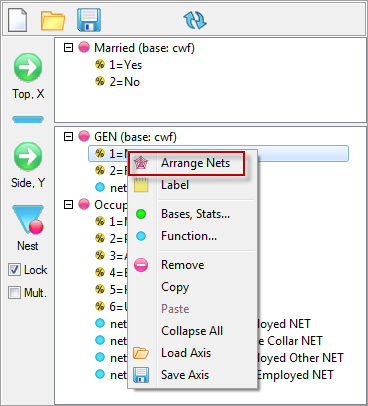
When selected, the NETs and codes in the specification are rearranged as follows:
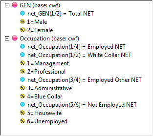
When the specification has the NETs arranged, the change is permanent.
Toggling the Arrange Nets off, from the report labels' context menu, will just removed the indenting of the subordinate labels, as seen here:
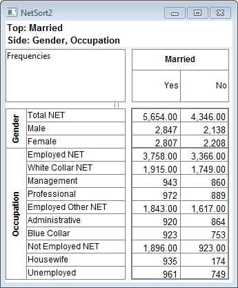
Label
In most context menus where variables or codes are found (in the variable tree, on tables and charts) there is a Label item ...
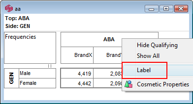
… which opens the Expression and Label form:
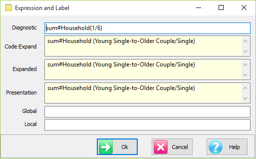
The fields correspond to the label modes showing all four automatic forms (read only) and offering two possible presentation texts:
Global text applies to this variable or code or expression on all reports in this job.
This is most useful for job wide filters so something like 'GEN(1)' is replaced everywhere by 'Males'.
Local text applies to this instance of the report only.
There are functional differences between the label for a normal code or variable and for a function or filter.
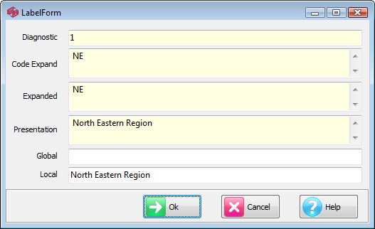
For a normal code or variable the fields show the Diagnostic (the code number '1'), Expanded (label 'NE') and current Presentation text ('North Eastern Region').
There are two fields in which you can enter Global and Local Presentation text:
Global text will apply to all uses of this code on any report in this job - these are stored in the Job.INI file.
Local text will override the global value for this report only - these are stored in the report file itself.
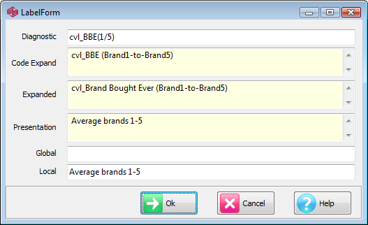
For an expression, as pictured above, the Expression field can be edited.
The expression may be for a function node in a table specification or a filter or weight.
Again the Presentation text can be Global (all reports in this job) or Local (just this report)
Presentation mode represents the highest level of labeling.
In this mode the label will come from the highest available in the following sequence:
Local presentation text
Global presentation text
Variable description or code label
Variable AKA or name, code number
Leading text in code labels or presentation text is preserved into exports so you can organise indenting of labels.
The leading spaces inserted into a code label...
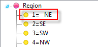
...persist into the table...
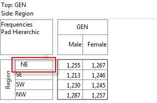
... and into Excel.
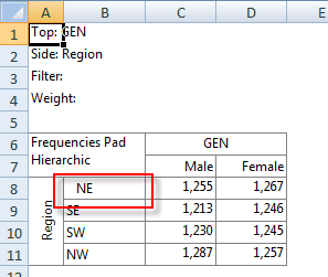
Data
Ruby case data items are numeric because the essential business of Ruby is running cross tabulations and a cross tabulation counts the number of numbers.
Data can be single response, multi-response, hierarchical, incremented or any logical mix thereof. Codes can be any real (float or double) number expressable within 16 significant digits.
Text data is accommodated by storing the text as an integer codeframe, so in effect text data is fully supported too.
Calendar case data is stored in Modified Julian Date format, which is the number of days as integer since 17Nov1858 - see Handling Dates
The Data menu item is available anywhere variables are displayed.
This form shows the data for each case in the selected variable.
The Specification form is probably the most familiar place to inspect data but any form with a variable tree will do.
Open the Specification form
Right click on UBAN and select Data
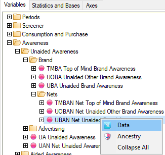
This shows the data for each case as
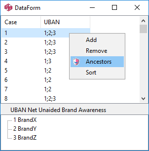
Click on anything in the UBAN column and the data is de-coded in the bottom panel.
You can also automatically add one level of ancestors to a constructed variable with the Ancestors item.
Right-click in the UBAN column and select Ancestors, as shown above, and then again on the UBA column to see its two ancestors in turn
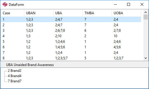
Resize the columns to suit.
Clicking on an item in any column shows the data for that variable in the bottom panel.
This is an excellent way to check if constructions are correct.
See also Ancestry Form.
The context menu is
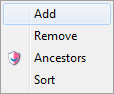
Add: Add allows you to add one or more other variables - you can multi-select in the file selector to add many at once.
Sort: Sort the data on any column.
Right-click on the TMBA column and select Sort
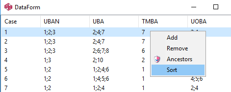
Note the cases are now sorted by the brand code, lowest to highest.
You can also see the codeframe for any variable by clicking on the column header.
Click on the UBAN column header
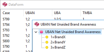
The codeframe form may additionally show the Expand button for codeframes that are duplicates of another, or are self-coding.
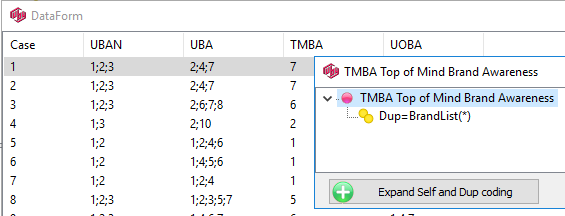
This form is very useful for decoding variable hierarchies.
Close the Data form
Find BratRats under the Image and Attributes folder and select Data
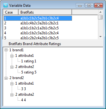
The lower panel shows the code labels and the hierarchic structure as a tree.
Ancestry Form
This form is for tracing construction ancestry all the way back to the source variables.
Right click on the variable A (constructed from all types of awareness) and select Ancestry from the right-mouse menu
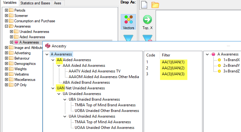
The left panel shows the variable as a tree with all other variables it depends on as children. A is constructed from AA and UAN, which are in turn constructed from AA and ABA, and UA, which in turn are constructed from various Awareness source variables as the tree shows.
Click on any non-leaf node to see its logic in the middle panel.
Click on any node to see its codeframe on the right.
All variable nodes have a Data item so that you can follow through the complete logic for any given case.
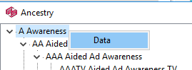
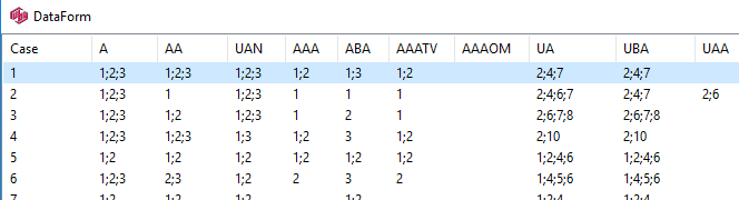
See the Data Form for details.
The construction tree can be saved as a text file.
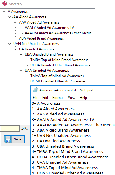
The depth of the tree node is indicated by the initial number followed by the variable name and its description.
+ and - indicate if the node is expanded (+) or collapsed (-).
Insert Statistics and Bases
Selecting Bases, Stats… from the right mouse context menus on the Top/Side trees of the Specification form opens the Insert Statistics and Bases form.
This offers a quick way to add extra nodes to variables in the Top or Side tree.
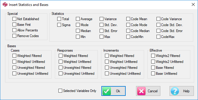
The Statistics and Bases groups generally correspond to the Statistics and Bases tab on the Specification form.
Any checked switches will cause that statistic or base to be added to all or selected variables in the Top or Side tree as if it had been dragged from the list.
The other check boxes are:
Special | Base First: has the same effect as selecting the Base First menu item on every variable.
Special | Allow Percents: is the same as double-clicking every added base or statistic to toggle the % sign.
Special | Remove Codes: removes all codes, leaving bases, statistics and expressions (convenient for quickly creating T2B/B2B and mean summaries).
Selected Variables Only: Apply the change to the selected variables only.
There are some ambiguities of definition:
Total is often used as a base but is classified in Ruby as a statistic.
Weights2 (meaning sum of squared weights) is classified as a statistic but appears here in the Bases section because it is primarily used to calculate the effective Base.
Function - Expression Builder
To build an expression in either the Top or Side panels, right-click in the panel and select Function...
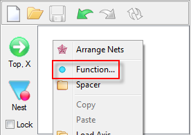
The Function menu item opens the Build Expression form where you can build an expression using drag/drop from the variable tree and insert logical operators with button clicks.
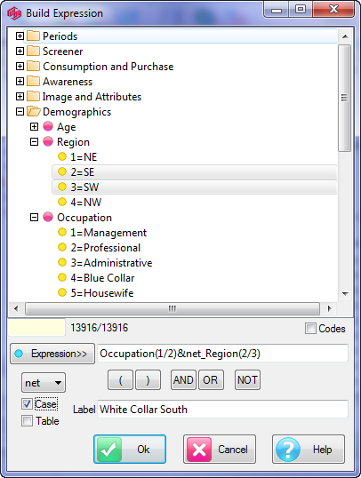
Along with the normal drag/drop behaviour, and case-level functions like net, there are the conventional buttons for building complex filter expressions.
You can also add a label for the expression at this point.
Dropping anything in the expression field will automatically add a '&' if there is no operator at the end.
Clicking any of the buttons will insert that character at the cursor.
Spacers
Spacers are used to separate sections of a specification as optionally labeled blank rows.
Start a New table
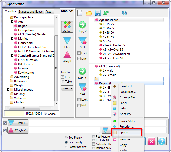
Drag Age to the Top
Drag Gender and Region to the Side
Right-click on Region and select Spacer - the spacer node is inserted before the highlight point and appears as a folder with text as “---”.
Click Run
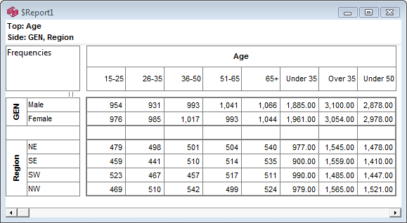
The Spacer appears as a blank row or column.
You can give the row a Presentation label in the normal way using the Label menu item in the Specification form or directly on the table.
Spacer text will always show as specified regardless of the current label mode.
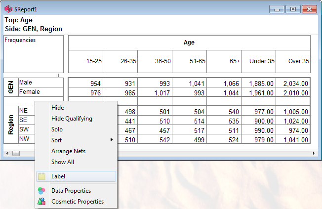
Variable Tree - Variable Context Menu
The context menu for a variable for the Variable tree is:
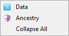
If you are over a code with Callouts, the menu is extended so you can 'play' any files attached to the code.
Any code of any variable can carry meta-data, including file attachments.
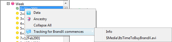
Data: Opens the Data form that shows you the case data for the selected variable.
Ancestry: Opens the Ancestry form that shows you the construction ancestry of the selected variable.
Collapse All: Collapses all open branches.
Hierarchic Specifications
Ruby fully supports variable hierarchies to any depth.
The most common hierarchy is a grid variable such as ratings within a set of parent categories (brand, statement, customer service, etc).
Unlike most tabulation specification systems, all levels of the hierarchy can be tabulated simultaneously against other variables. For details see Processing Hierarchies.
Hierarchic variables are identified by their structural representation.
Here is the specification for week by BratRats, which is a brand/attribute/rating cube or Level C hierarchy.
Start a New table 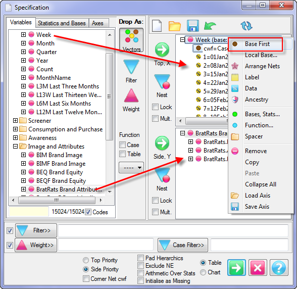
Drag Week to the Top
Select Base First on Week
Open Image and Attributes and drag BratRats to the Side
Open BratRats on the Side specification tree to see the hierarchy
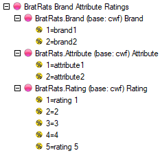
The hierarchic levels are nested under the parent name.
You read the hierarchy top down as for each brand there is a set of attributes, and for each attribute, there is a set of ratings.
The actual number of vectors which will be supplied as table rows is Brands x Attributes x Ratings, 2*2*5 = 20.
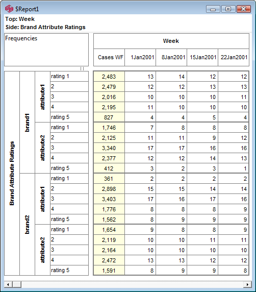
Note how the nesting on the side labels matches the structure of the hierarchy.
Each level can be tabulated as a separate variable.
Home New
Open the BratRats variable in the Variable Tree
Drag BratRats.Brand to Top
Drag BratRats.Attibute to Side
Open the Ratings level
Drag BratRats.Rating(1/2) to Filter
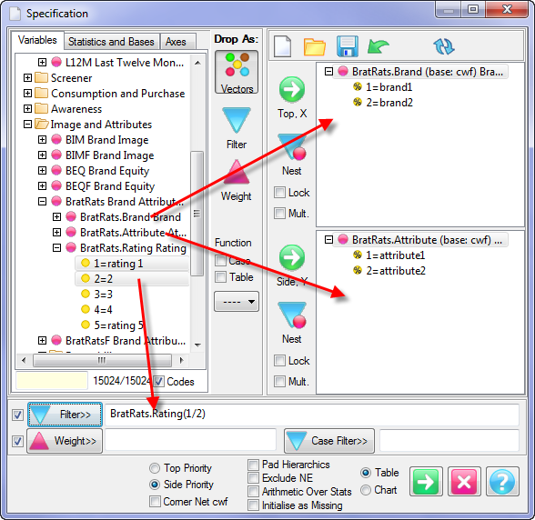
Click Run
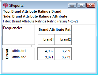
This table shows the counts for top-box ratings 1 and 2 only.
You can tabulate any hierarchic level against any matching level of another variable, or against any flat variable. If against a flat, then the level is processed as if it were a multi-response variable.
If there is a mismatch in the case data structure you are warned as each mismatch is encountered:
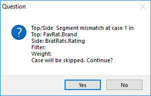
If the specification is correct, then a mismatch usually indicates a data collection issue such as inconsistent questionnaire jumps resulting in unexpectedly different brand sets.
For example, consider a bank of variables all asked of the same set of brands, usually determined by a prior awareness or usage question:
var1: a1b2a2b3a3b4
var2: a3b5a4b6
var2 is missing the third A level node so the hierarchies at this case are not compatible.
Drop Modes
Drop As:
The three big buttons - Vectors, Filter and Weight - exclusively switch the Drop Mode, which determine what happens when you drop something on the Top and Side panels.
Normally you drop Vectors (rows or columns) but you can also drop local filters and weights from the variable tree.
Function:
Regardless of Drop Mode, you can arrange for dropped variables and codes to turn into Function expressions.
If the Case Function or Table Function switch is ON, then the function selected in the respective drop down list is used.
In the Spec form below:
The Top axis began as Occupation dropped as Vector, then WghtAgeGenRegCell was dropped on Occupation as Weight, and then GEN(1) dropped on the weight as Filter.
Side had the Table Function sum checked, resulting in sum#Age(1/3) appearing in the Side panel under the Age variable.
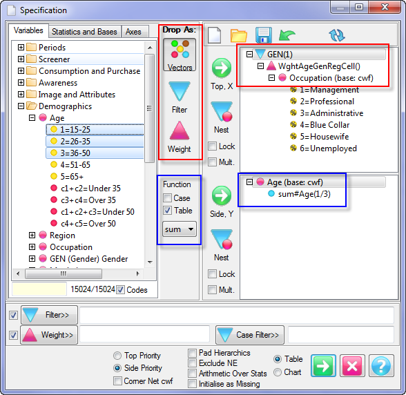
Filters and weights within an axis are called local, as opposed to the table-wide filter and weight at the bottom of the Specification form.
All local and table filters are ANDed, and all weights are multiplied, for a final per-case true/false and weight value.
Case Functions and Expressions
Case functions operate on case data.
For example, if a multi-response variable like NumTimes has data for a case as 1,2,3, then the function sum_NumTimes() returns 1+2+3=6.
All case functions can be scoped for code, so that:
sum_NumTimes(1/2) returns 1+2=3
sum_NumTimes(1;3) returns 1+3=4
sum_NumTimes(1) returns 1=1, that is just the code itself
sum_NumTimes(*) returns the sum of all response codes defined in the code frame, here 1+2+3=6
sum_NumTimes() returns the sum of all response values, whether in the codeframe or not, and if uncoded, then all values.
To demonstrate,
Start a New table

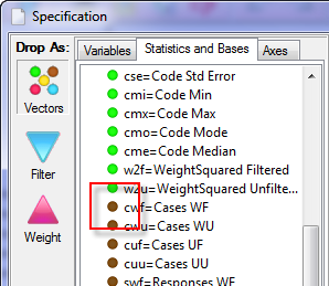
Make sure there are no default stats or bases by double-clicking on any to cycle through the states
Drag Week to the Top
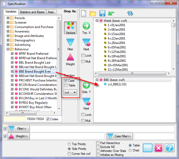
Set the function settings as indicated - check Case and select cvl from the drop down
Open the Behaviour node and drag BBE to the Side
Notice the result is a single blue node under its codeframe. Here, the function cvl - Count of Values - has been selected, which returns the number of values at each case of the selected variable.
With Case checked, and a function selected, a code selection for Top or Side now results in the function expression.
Click Run
Set Decimals for Expressions to 0 in the Properties | Cells tab
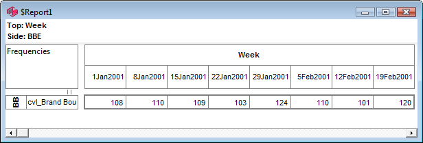
So in the first week, among all respondents, there were 108 brands mentioned.
To change to percentages.
Respecify
Right-click on BBE and select Base first
Double-click on the cvl_BBE function node to toggle showing percents
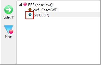
Click Run

When the table appears toggle Column Percents ON from the Home page of the ribbon
This tells us, for instance, that in the second week, on average each respondent bought around 2.2 brands.
You can actually change the display to report 2.2 instead of 220%.
Open the Properties form
On the Flags tab set Force Percents to Proportions ON
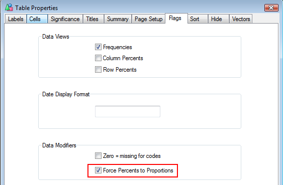
On the Cells tab set Percents decimals to 2
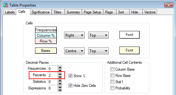
Click OK
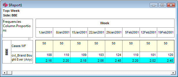
Case expressions can be edited. If you want to restrict the count to just the number of brand codes 1 to 5 then the cvl_ expression can be modified.
Respecify
Right-click on the function and select Expression and Label
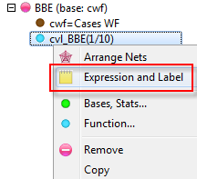
Change the Expression field to cvl_BBE(1/5)
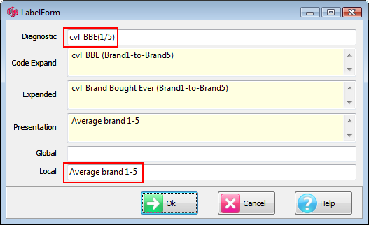
Optionally, add a Local Presentation label for the function
Click Ok
Back in the Specification form click Run
Select Presentation from the Display Status group on the Home tab. This makes the customised label for the second row show:
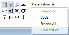
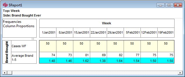
The counts are reduced by about a third.
Limiting the scope of a function is very convenient when the codeframe is something like 1, 2, 3, 98, 99, and you want to exclude the 98 and 99 from consideration.
The Case functions appear in a drop-down list in the Specification form when the Case function checkbox is selected.
Most of these are sensible for multi-response data only.
Only the cumulative sum function works across cases.
All case functions return a value for each case which is utilised as appropriate by the crosstab algorithm.
You can use standard arithmetic operators and constants, so 10*cvl_BBE(*) would multiply the number of values by 10.
Table Functions and Expressions
The Table functions appear in a drop-down list in the Specification form when the Table function checkbox is selected.
Table functions are specified in the same way as case functions, except that Table is checked instead of Cases, and when dropped, the function has a # instead of an _.
The mnemonic is that _ is the lowest character, hence a case operation at the lowest level, and # looks like a grid, hence table level.
Although many of the names are the same as for Case functions, the operation is quite different because Table functions work on the vectors of the table itself after it has been generated.
Exercise: Using the Table function
In this hands-on exercise you will use the Table function 'sum'.
Start a new table
Drag Region to the Top
Drag Occupation to the Side
Set the function by checking Table and selecting sum from the drop down
Open Occupation on the right and multi-select codes 1-3
Drag to the Occupation variable in the Side panel
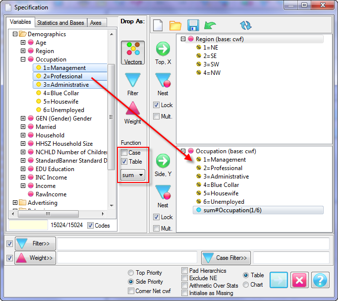
Click Run
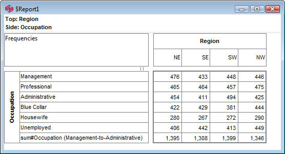
Looking at the NE column, 1,395 = 476+465+454, showing that the last row is the sum of the first three.
The Insert Function
The ins function is different from all the others in that it does not derive values from variables and codes.
If you select this function it doesn't matter what you drag across or have selected when you click a Top/Side button, the result will always be to open the Expressions form where you add explicit numbers.
The purpose is to allow entering explicit numbers that might be reference values, norms, or even data that is unrelated to the cases in your job.
To insert some non-survey data to the previous table:
Respecify
Set the function controls on the left to Table and select the ins function
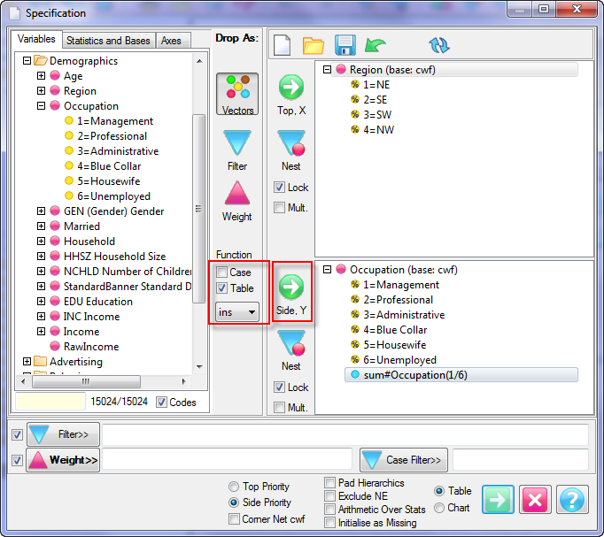
Click the Side button - the Expression form opens
Change the Expression field to ins#(1200;1100;1000;1300)
Note that the separator is a semi-colon. The semi-colon is used to prevent confusion with the European use of comma for a decimal point.
You enter one number for each column - if there are less numbers than columns the remaining columns have missing data.
Change the Local label to Last Year
Click OK
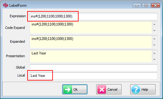
Click the Side button again to add a second insert
Set the Expression field as ins#(#1200)
The constant 1200 is inserted to every cell in the row. If the first character after the open bracket is a # then that number is propagated along all columns.
Change the Local label to National Average
Click OK
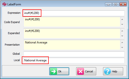
This produces the following Side specification:
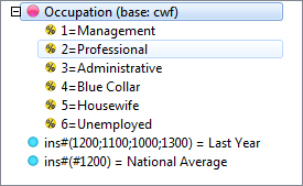
Back in the Specification form click Run
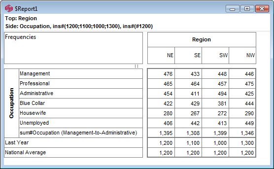
Note that the second last line is filled with the varying numbers from the first ins function, and the last line is filled with four instances of the same number.
Percentiles
Table Medians and Code Medians equivalent to the 50th percentile.
If you want other thresholds, use the PCL (Percentile) and CPL (CodePercentile) functions.
These are a bit like the INS function in that you'll probably want to edit the expression that is dropped.
Exercise: Percentiles (pcl)
Start a new table of Region by TMBA
Select Table Functions and the pcl function
Drop TMBA on the side
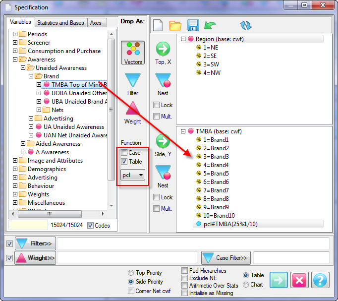
The default is 25th percentile over all codes (or whatever code selection you made).
Right-click on the expression and select Expression and Label
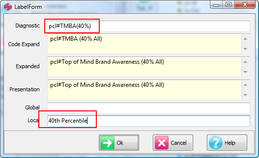
Change to the desired percentile (do not remove the % - this is the key character that indicates this is a percentile) and change the code range expression if you want.
In this example the expression has been removed altogether but you might want to exclude some codes in a more complicated variable.
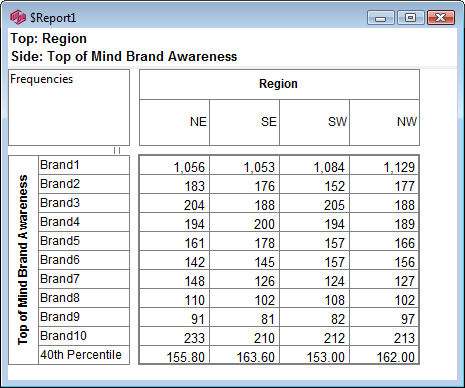
The resulting table has interpolated figures that represent the threshold below which 40% of the values will lie.
Percentiles can be calculated a number of different ways.
One common method is: in N items the pth percentile is item p(N+1).
Excel uses a different formula: 1+p(N-1).
Ruby's default is the common formula but you can switch to match results from Excel at Preferences|Job Settings.
Exercise: Code Percentiles (cpl)
When you have a variable whose codes are actual values you can use Code Percentile.
Start a new table of Region by Income
Select Table Functions and the cpl function
Drop Income on the side
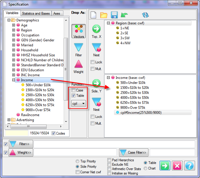
Run
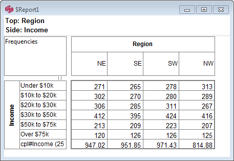
The table shows the 25th percentile for income in each region. Because the codes are actual income values the percentile is also.
Specify Banners on the Fly
The simplest banner is made by dragging the variables you want to Top.
Start a new table
Drag Age, Region and Gender to the top
Drag BPRF to the side
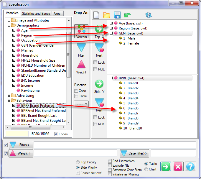
Click Run
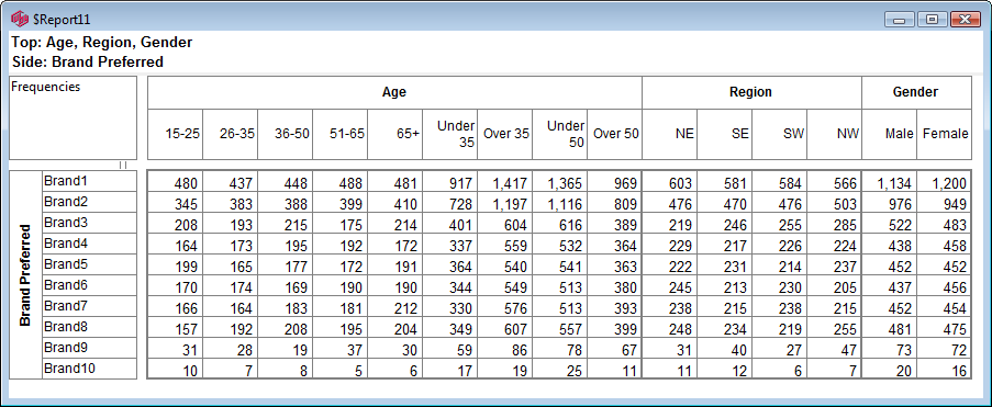
Specify Nets on the Fly
The Age variable has some inbuilt nets (implemented as code arithmetic) that are a permanent part of the variable. These were specified in the Edit Variable form as part of the job setup.
This exercise shows that net and sum are equivalent operations for single response variables.
Start a new table
Drag Age to the top and Occupation to the side
Delete the last three Age code arithmetic arithmetic expressions (retain c1+c2 for comparison)
Select Case functions and in the drop down select net
Multi-select the first two codes of Age and drag them to the Age variable on the top
This creates a blue function node under Age that is the net of codes 1 and 2.
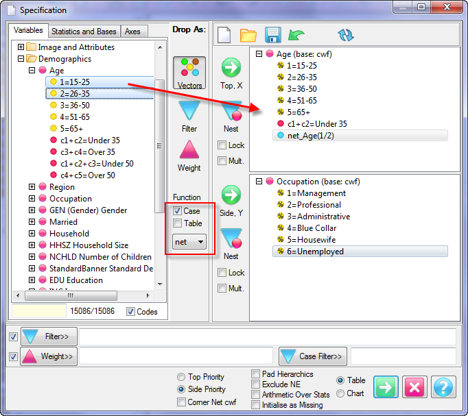
Click Run
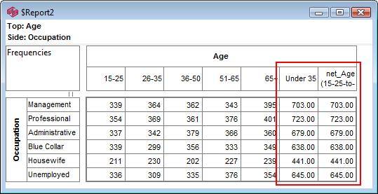
The last two columns are identical showing you that if there is not a net already in a variable you can make one on the fly in the Specification form.
Since net_ works at the case data level, and sum# and code arithmetic work at the generated table level, table arithmetic (vector operands) is usually hugely faster.
For this reason you should always consider for single response data whether a sum# or code sum is sufficient.
For multi-response data, net_ avoids double counting, so you cannot end up with a cases base count which exceeds all respondents.
Specification Files
You can save a specification as a *.tbx ('table spec'), and use it as a template that can be reloaded when required.
There is an example in the supplied Demo job.
Start a new table
Click the Open button on the Specification form
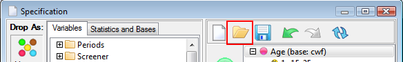
This opens the job's Specs folder showing *.tbx files.
Select StandardBannerSpec and click Open
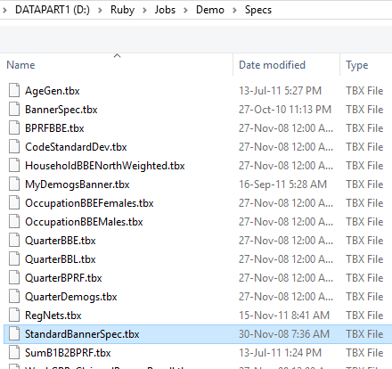
The top pane has a collection of variables with bases and expressions. You then supply whatever you want as the Side, overall filter and weight.
Drag BPRF to the side
Select Base First for BPRF
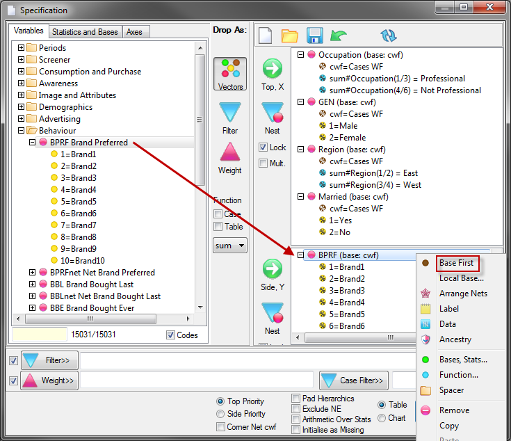
Click Run
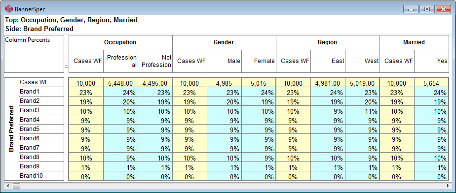
Make the table column percents only and Presentation mode on the Display Status group on the Home tab of the Ribbon:
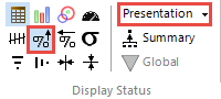
Note that the second column is labelled 'Professional' and yet appears as sum#Occupation(1/3) on the Specification form. This is because presentation text assigned locally to an item on the Specification form is saved in the .TBX file.
Advantages
Many incidental changes that a researcher would otherwise have to ask DP for can be done immediately by the researcher in the Specification form.
If you want Married as the left-most columns, instead of Occupation, then simply change the order for the top axis in the spec.
If you want to change the Occupation nets to Management vs All the Rest, then you can directly edit the Expression to a different range or codes by right click and select Expression on the sum#Occupation nodes.
If you want to expand the banner with another demographic, then simply add it to the Top spec tree.
You can run the banner across many variables and make a table for each using the side Multiple switch.
A TBX file is a more general version of Axes, since it covers all specification items (top, side, filter, weight).
Axes and the Axes tab
Any axis can be saved in the Axes tree for later use, from the right mouse context menu.
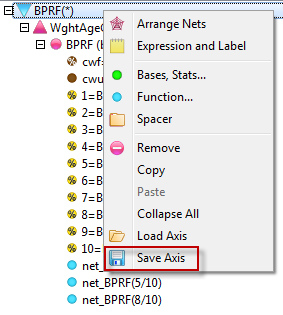
The Save dialog box appears as follows:
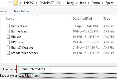
The axis, containing any filters, weights, expressions, nets etc. can now be dragged and dropped into Side or Top of a report specification, just as you would do with a variable.
With the Details checkbox ticked, you can see the structure of the axes.
Where a complex arrangement is reused axes can save time and reduce potential for errors.
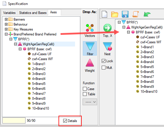
Filtering a Table
Any table can have an overall filter.
The filter is created by dragging codes to the Filter field at the bottom of the form, or by entering or editing filter expressions directly.
The default is to OR codes, and to AND variables.
If you want something different, such as nestings like ((A&B)|C)&~D, then you drop the variable(code) components represented by the A, B, C and D, and then edit the expression manually.
To filter a table on Household (Young Single;Peer Group;Young Family)
Open the Household variable
Multi-select codes 1/3
Either drag to the Filter field, or click the Filter>> button
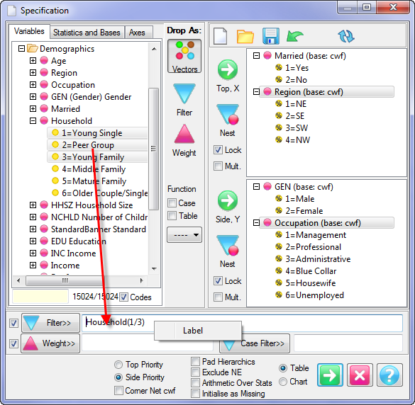
Note that the filter is represented in its lowest form - variable name and code numbers. This makes it easy to edit manually.
You can decode the filter into its full text form at any time from the Label item on the Filter right mouse context menu.
Click Run
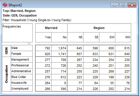
The cell contents have all reduced by about 50%, and the filter is displayed using code labels as Household(Young Single-to-Young Family).
The filter can be temporarily turned off without losing the specification by unchecking the check box to the left of the filter button on the Specification form.
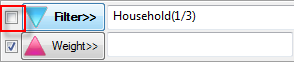
Exercise: Nested Filters
Nesting splits a specification axis once for each selected code (or all codes).
To nest a Side axis on Gender
Select Gender in the Variable Tree
Click the Side Nest button
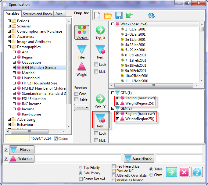
The above shows the Side branches open to make clear that the entire Side specification as it was has been duplicated and locally filtered to each of the codes of Gender in turn.
Click Run
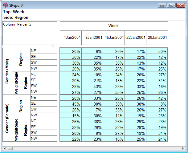
Notice that the nesting of the side labels makes clear where local filters and weights have been applied. Local weights, local filters and nested filters can be layered to any depth, and can be organised in any way that makes logical sense.
The filter expressions can be manually edited at any time via the right mouse menu Label item.
Optimising Case Filter vs Global Filter
There are two overall filters that can be employed and they are for different purposes.
The Global Filter is set on the Preferences form and toggled on/off from the ribbon to force a filter on every report that is viewed. The Case Filter is on the Specification form and is an optimising filter that simply excludes all non-matching cases from the table altogether - usually to achieve faster runs.
The Global Filter
You can set a Global Filter in Preferences Job Settings and turn it on/off on the Display Status group on the Home tab of the Ribbon.
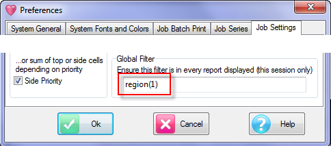
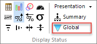
This filters every table as it is opened or displayed - so new reports and opened reports will be filtered to the Global Filter.
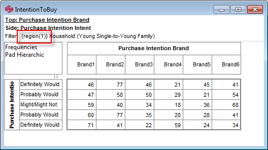
The Global Filter appears in curly braces in the filter display.
The Case Filter
Setting a case filter produces much the same result.
Here the case Filter is set to Region(1), NE Region
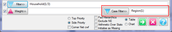
The Case Filter also appears in curly braces but with dashes as well.
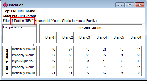
The difference can be seen in the generation times.
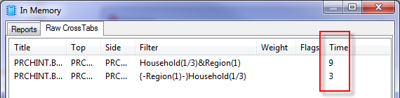
The first crosstab has Region(1) as a conventional filter and took 9 centiseconds.
The second has Region(1) as a Case Filter and took 3 centiseconds.
This is because the second table only processed cases that matched Region(1) - the first table includes 10,000 cases and the second only ~2500.
This is very useful for things like looking at a short time period in a large continuous job.
It is not suitable if you want all cases processed so they appear in unfiltered bases.
Weighting a Table
Any expression which can be evaluated to a single value (or, if hierarchic, a hierarchic level of values) can be used as a weight.
The common use for weighting in survey data is to specify a variable that smooths out irregularities in the sampling according to some target quota scheme.
However, the concept of weighting in Ruby is very flexible. A variable is a weighting variable only by application, not by definition.
This means that you can weight a table on just about anything, from a single-response variable like Gender to the sum of multi-responses to any complex expression, or by quantitative data such as price paid to get aggregated expenditure.
To apply a weight, simply drag the variable to be used as a weight to the Weight field at the bottom of the Specification form.
Open the Weights folder, select WeightGenRegCell and either drag it to the Weight field or click the Weight
 button
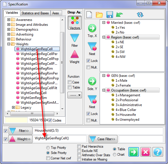
Click Run
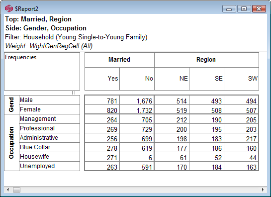
The weight is displayed as the last line in the table's Title region.
The weight can be temporarily turned off without losing the specification by unchecking the check box to the left.
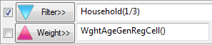
Note that the weight is supplied as WeightGenRegCell (), with parentheses, and not just as WeightGenRegCell. This is because weights are always implied sum_ expressions, and often it is useful to be able to scope for the data which will be used for the weighting operation.
If you wanted to weight on a variable xyz with a code frame of 1, 2, 3, 99, where 99=None/Don't Know, then the 99 can be eliminated without explicit filtering by specifying the weight as xyz(1/3). If xyz is multi-response, then the weight factor will be the sum of codes 1 to 3 for each case.
Weights can be a hierarchic level. This table shows the sum of ratings for each Brand/Statement.
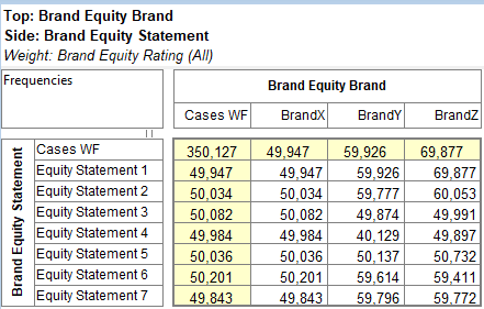
This can be especially useful for volumetric tables.
If the hierarchic level has multi-response segments, then the weight per segment is the sum of the codes.
Local Filters and Weights
Any variable in the Top and Side trees can be locally filtered or weighted. This is done by selecting the Drop mode as either Filter or Weight.
Change the Drop Mode to Filter by clicking the big top left Filter button
Open Occupation and drop code 1 on any part of Region in the Top axis
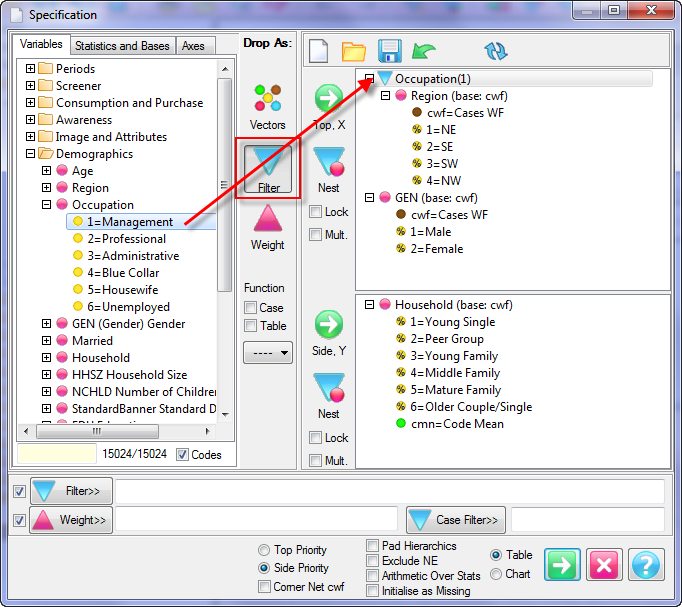
Click Run
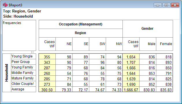
Notice how the nesting of the top labels indicates that the first block, Region, is filtered and the second block, Gender, is not.
These local filters are in addition to (ANDed with) any table wide filtering.
Similarly, with the Weight drop button depressed, drops on the specification tree insert a weight, and the weight value will be multiplied by an overall table weight if one is present.
To see Region both weighted and unweighted in the same table:
Home New
Drag Week to Top
Drag Region to Side
Drag Region to Side a second time
Change the drop mode to Weight by clicking the large Weight button
Open the Weights/Legacy folder
Drag WeightRegion25 to Side and drop on any part of the second instance of Region
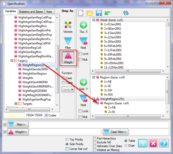
Click Run
Set display to column percents only:
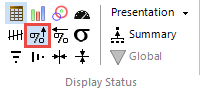
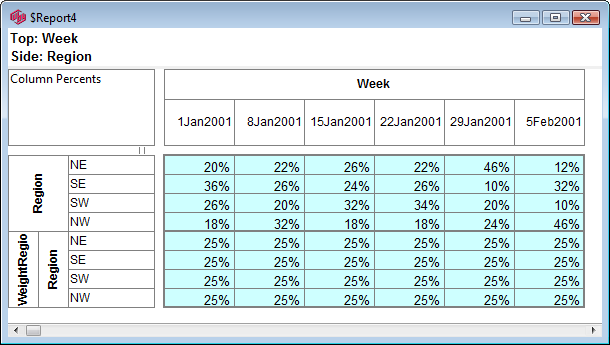
As expected, since the weight is WeightRegion25 and the weights are calculated within weekly, each weighted cell is exactly 25%.
Presentation Text
Any labels you have added for presentation purposes are visible on the Top and Side specification trees.
If there is a space before the = sign it means presentation text after the = sign.
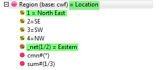
See Label Modes.
Run Time Flags
The run time flags are
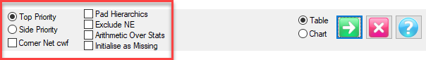
These properties need to be set before table generation, that is, they apply at run time, not at display time.
Top/Side Priority: Give the top or side axis priority for the cell value at intersecting base and statistics. See Priority at Intersections for details.
Corner Net cwf: Show the total headcount at the top left corner rather than the default sum-of-values in the priority direction. See Corner Net Respondents for details.
Pad Hierarchics: Pad missing nodes in hierarchic variables with virtual Not Established. This pads up the base counts to what would have been obtained if using flat source or breakouts of the hierarchy. See Bases and Pad Hierarchic Data for details.
Exclude NE: Remove Not Established values or cases from the base counts. This is usually the same as filtering to valid codes on both axes. See Bases and Excluding Not Estabished for details.
Arithmetic Over Stats: The default is to do statistics of the arithmetic. This flag reverses that, as arithmetic of the statistics. See Priority at Intersections for details.
Initialise as Missing: Initialise table cells as missing rather than the default zero. This is useful for time series charts to show zero points as a gap.
The Specification form has a set of switches for controlling table generation.
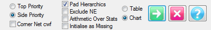
They have job-wide counterparts on the Preferences form, representing the defaults for a new table specification.
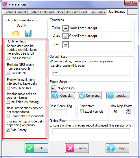
Top/Side Priority and Corner Net flags are also on the Properties|Flags tab but can be set here before the run.
Vector Priority
Table cells are the result of a row and column intersection and there are some cases where priority is required.
A row/column vector could be:
The default priority sequence is as listed above.
Functions are highest so if a row or column is a function node in the table specification then all cells will be from that calculation.
Next is Stats, above Arithmetic, so the first table below is what usually happens in Ruby.
The yellow highlight cells below are the result of the Stat column (avg) - ie 96.53 is the average of the region code1-4 cells along the row: 94.96, 93.33, 105.66 and 92.18.
If you want this to be the other way round you can set Arith Over Stats ON and the second table will result.
The first yellow cell is the result of the row Arithmetic expression #100*c1/avg - ie 96.50 = 100*482.5/500 from the age code 1 and avg cells in the column.
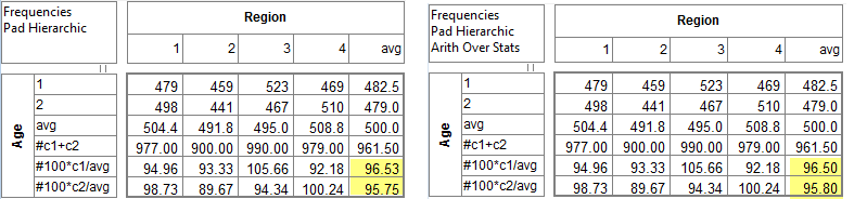
There are three arithmetic rows - a simple sum and two index calculations - and a statistic column.
In the first table the yellow cells are averages - ie 95.75 is the average of the other cells in the row (column expression avg is used).
In the second table the yellow cells are index calculations - ie 96.50 is 100*482.5/500 (row expression 100*c1/avg is used).
Priority at Intersections
Ambiguous cells can arise with multi-response and other complex data where the top base and side base intersect - do you show the total count of responses or cases?
Similarly, if Cases WF and Cases UF, does the intersection show weighted or unweighted?
The first table shows 10,000 (total cases) in the top left cell because priority is with the top variable, which is a simple single response.
The second table shows 34,027 (total responses) in the top left cell because priority is with the side variable, which is multi-response.
Note the 'equal' sign in the gap indicating which way the addition is done to produce the result in any intersecting base cells.
Intersecting base cells default to the sum of bases in the indicated direction, unless (for Cases Weighted Filtered) Corner Net cwf is ON.
This is one of the Table Flags that can be set prior to running a table...
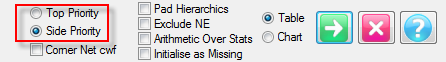
... and it is also setting is on the Flags tab of the Table Properties form that can be changed after the table has been run.
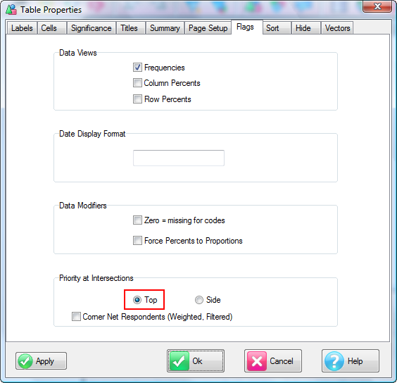
If you want column percentages simultaneously on both 10,000 and 34,027, then supply Count as the first Top variable, and set Priority to Side.
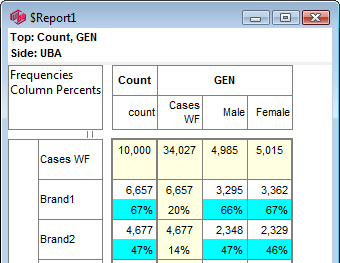
The Priority settings also determine the way in which the standard statistics are calculated.
If a table has Total on one axis, and Code Mean on the other, then an intersecting cell could show either the total of the means, or the mean of the totals.
Total of means=1.5+1.51+1.5+1.49 Mean of totals = (4985+5015*2)/10000
=6.01 = 1.5
To show weighted and unweighted base rows against a weighted base column, set the priority to Top.
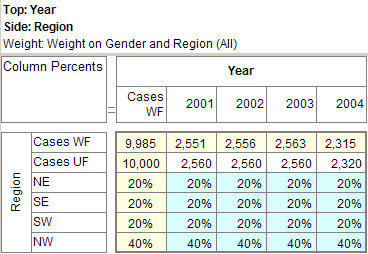
Corner Net Respondents
The Corner Net flag can be set in two places:
On the Specification form...
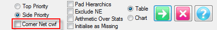
...or in the Flags tab of the Table Properties form.
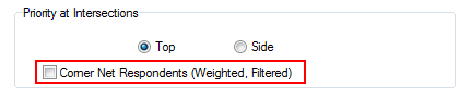
The other switch here only affects the fixed base (yellow) intersections.
If you want the corner cell to always be Net Respondents set this switch ON.
The Net value will then be used for percentaging bases and statistics that use the corner value (e.g. Single Cell).
ArithOverStats flag
If the table has both arithmetic and statistics vectors, then there will be two possible values for some cells - the arithmetic of the statistic, or the statistic of the arithmetic.
The simplest demonstration is a table with a code mean column and an arithmetic constant as a row:
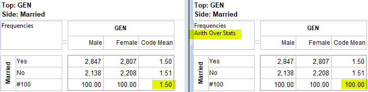
For the table on the left, the code mean has priority. This is the default behaviour. For the table on the right, the arithmetic constant expression has priority over the statistic.
This is useful for any circumstance where you want the sum of a statistic, such as code variance or weights squared. For example
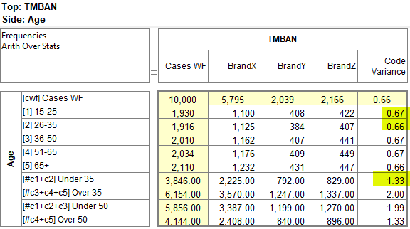
The variance for Under 35 is calculated as c1+c2=0.67+0.66=1.33.
Sum of wghts^2 is a common manoeuvre. Weighting by 10, with Arith over Stats OFF, the bottom right cells cannot be calculated:
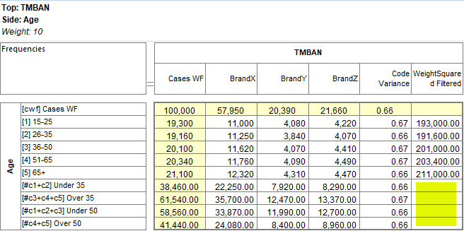
With Arith Over Stats ON, the cells can be populated:
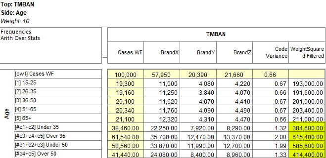
For other applications of this flag see Indexed Reports.
Basing a Table
In Ruby, a base is any vector created by any means to be used as the denominator for a percentaging operation. A base is not a filter, though it can be the result of a filter.
Every percentaging variable should have an assigned default base - for survey data the most common base type is Cases Weighted Filtered (cwf).
Only one base can be used for percentaging under each variable, but any other base can be displayed.
There are fourteen standard bases which are always aggregated at cross tabulation time, and so are always immediately available.
The default base is set on the Job Settings tab of the Preferences form.
cwf (Cases Weighted Filtered) is the most common default.
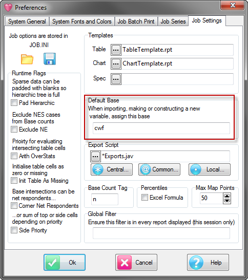
In the Specification form right-clicking on a variable displays a menu where Base First will add the default base to the variable.
The brown cwf code is inserted after the variable.
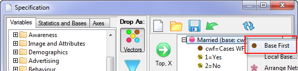
By default, the inserted base will not display percentages, but double-clicking the brown circle will enable percentaging.
Note that the Base percentage of itself is 100% and will not display in the table (because redundant), even though percentaging the base is enabled.
The following table illustrates this:

Add Other Bases
The Statistics and Bases tab displays the available bases.
The top four bases have been multiselected and dragged to Gender on the Side in the Report Spec shown below.
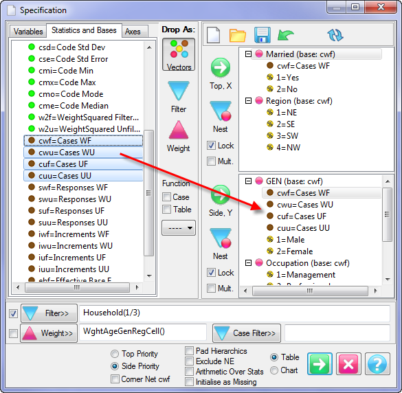
Note that the default base for GEN is cwf and that cwf is the first base.
This means it will show on the table with a yellow background indicating that it is the percentaging base.
The rules for showing the background for a percentaging base are:
It must be the designated base for this variable - indicated above as (base: cwf)
It must be the first item after the variable node.
You can percentage on a base no matter whether it is displayed or not, and no matter where it is in the table, or even if in another table altogether, but the base background colour only displays if the base is the first row or column for the variable.
This is because bases can be locked against scrolling (like freezing panes in Excel) so that they are always in view - not possible if the base could be anywhere.
The table below displays Column% only, as set by the button on the Display Status group on the Home tab:
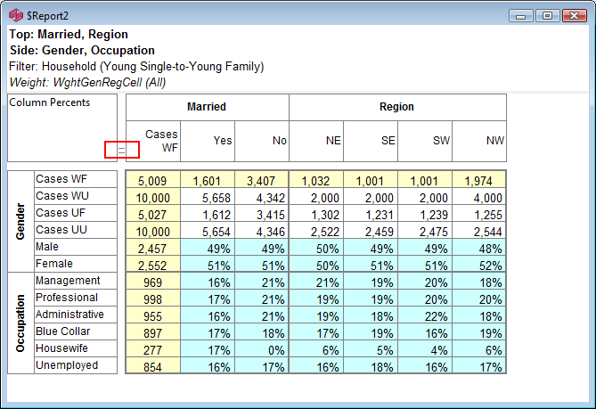
Note the 'equals' indicator between the top left key area and the top labels. This shows the effect of the Priority flag.
The Priority flag determines which way around the sums are done for a cell that is both a Top and Side base.
This indicates that the first four cells in the first column, which are base rows as well as base columns, are the result of adding horizontally.
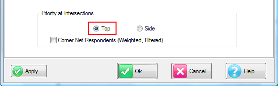
With a single response variable on both top and side, the Priority setting makes no difference.
For multi-response the Priority setting 'Top' will produce different values to Priority setting 'Side'.
Examples:
To see each of the non-percentaging bases as a percent of Cases Weighted Filtered (a good way to estimate the relative effects of the filter and/or weight):
Respecify
Toggle the percent status on all base nodes
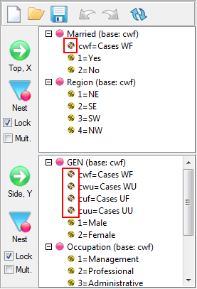
Click Run
Change Percents Decimals to 2 on the Properties|Cells tab
Resize columns if necessary to see all decimal places
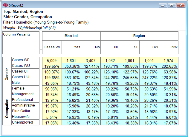
Bases and Pad Hierarchic Data
Hierarchic data is minimally stored.
A three-level variable could easily multiply out to thousands of potential nodes, with only a few or even none being used for any given case.
Only actualised hierarchic nodes are recorded on disk, thereby drastically reducing space requirements, but with the consequence that case data, which would otherwise (in a flat storage format) have contributed to the Not Established counts, is simply not present.
The effect is to auto-filter to valid (established) codes only, thereby reducing the respondent base counts.
Most of the time, this is the natural behaviour, but if you need to percentage on everyone, then the respondent base counts can be guaranteed to include Not Established by checking the “Pad Hierarchic Data” flag.
If set to ON, then sparse hierarchic data is virtually padded, at crosstab time, to be node-complete.
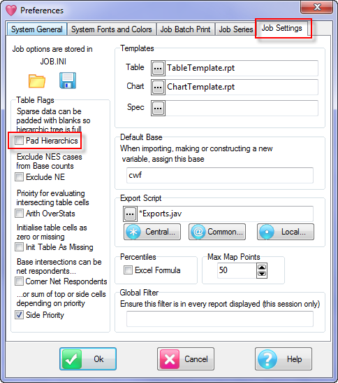
The job default setting is on Preferences | Job Settings and that can be overridden for any table with the switch on the Specification form.
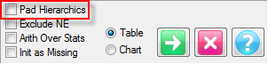
Step by step to demonstrate:
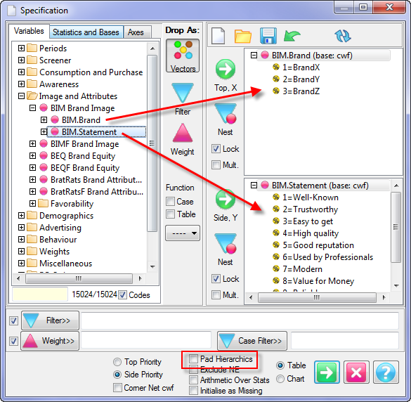
Ensure that the “Pad Hierarchic Data” flag is OFF
Specify the table BIM.Brand by BIM.Statement
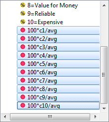
Delete the ten red index nodes in BIM.Statement: highlight, press [Delete]
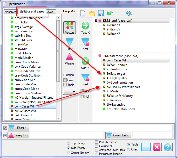
Switch to the “Statistics and Bases” tab
Drag nes and cwf on the side, click Run
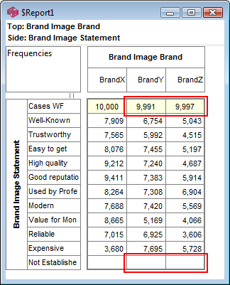
Note that the base for BrandY is 9 short of 10,000, and for BrandZ, 3 short. Thus, since there is no filter, it would be expected that the Not Established row would show 9 and 3. The Not Established row is in fact empty because of the auto-filtering side-effect of minimal storage, as explained above.
To get a base of 10,000 for each column, and the Not Established counts of 9 and 3
Respecify
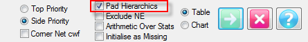
Turn Pad Hierarchics ON
The table is now
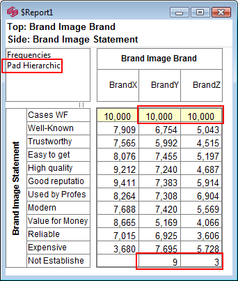
The base count is now 10,000 for each column, and the Not Established counts are present.
For jobs which often use percentages of respondents, the “Pad Hierarchic Data” flag would usually be permanently set to ON.
For jobs where the natural base is Totals, OFF may be more appropriate.
To remove the Not Established counts, so that percentages will be of those with a valid response only, respecify and apply a filter as BIM.Statement(*).
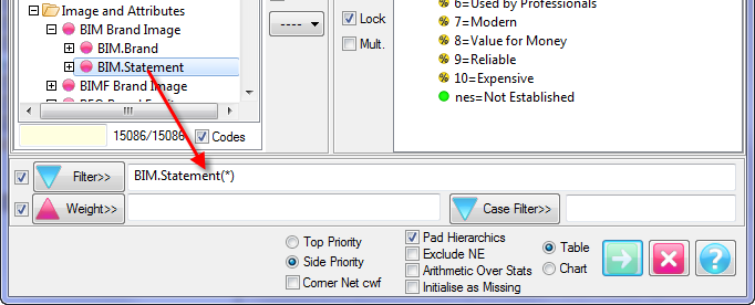
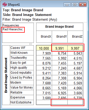
The base counts for BrandY and BrandZ have reverted to 9,991 and 9,997 because the Not Established data items inserted because “Pad Hierarchic Data” is ON have now been filtered out.
Leaving “Pad Hierarchic Data” always ON, and then filtering to remove the padded nodes, is probably the most intuitive approach for survey data because it matches what would be expected from flat storage.
For jobs which are all quantitative data (such as sales, scientific data, financial indices, etc) and the natural base is Totals, then OFF will give substantial improvements in crosstabulation speed for large hierarchies.
Bases and Excluding Not Estabished
“Pad Hierarchic Data” reveals all Not Established cases in sparse hierarchic data.
Sometimes you want the opposite - to exclude Not Established cases, and there are several ways doing this.
You could filter them out of the table altogether or merely exclude them from basing a couple of ways.
There is a job setting on the same tab as the “Pad Hierarchic Data” flag that does it simply.
Generate the table Region by Occupation with Not Established and bases on both top and side
Ensure that the “Exclude NE” and “Pad Hierarchic” flags are OFF
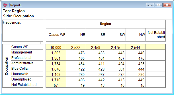
Notice there are 10-20 cases in each region that have no data for Occupation. Here are a couple of ways of removing them if desired.
Filter Out Not Established
Respecify the table
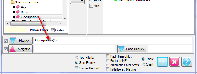
Drag Occupation to the Filter field
In the filter Occupation(*) the * means “valid codes” so any other cases will be excluded from the table entirely.
Click Run
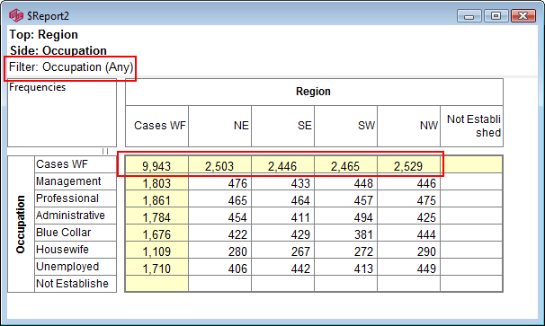
The filter is announced in the title area, the Not Established row is now empty and the bases have been reduced.
Exclude Not Established from Bases
Respecify the table
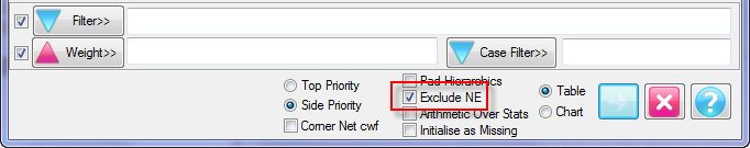
Remove the Occupation(*) filter
Turn “Exclude NE” ON
Click run
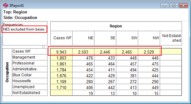
There is no filter line in the title field but there is advice in the key area “NES excluded from bases”. The column base counts have reduced by the invalid cases but their Not Established counts are still visible in the table body.
Note this only affects the brown-dot bases. Total is not one of those and will not be reduced even though it can be used as a base.
Other Techniques
Several DP techniques are available for giving individual variables special bases - like #cwf-nes to remove invalid cases explicitly.
Construction techniques can be employed to achieve similar results.
Select Base form
Clicking the Base button
 on the Variables form, or selecting the Local Base menu item on the Specification form, opens the Select Base form.
 This is for specifying the expression to be used for basing a particular codeframe.
Generally these are simple things like Cases or Totals but could be complex expressions.
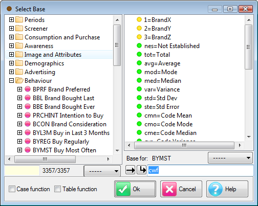
The similarity to the Arithmetic form is not accidental - bases can be assembled using all internal codeframe arithmetic.
Additionally, bases can be assembled the same way functions are assembled on the Table Specification form.
On the left is the variable tree.
On the right is the full target codeframe with the full set of pseudocode statistics and bases.
Under that is the name of the codeframe and the edit field holding the base expression.
Either drag things into here or use the two arrows at the left: the straight one brings in the selection for the variable tree; the bent one brings in selections from the codeframe.
A double-click in the codeframe display replaces the selection.
The two dropdowns with --- in their fields are for various algebras, as are the Case/Table function switches.
Simple bases
The example shows the simplest case where you have arrived at this form from the Edit Variable or Table Specification form, double-clicked on cwf to assign that as the base for Gender and are ready to click OK or press [Enter].
Arithmetic bases
If you clear the base field and drag code1 and code2 from the top right (either one at a time, or by [Shift] or [Ctrl] highlighting both then dragging the pair or clicking the bent arrow button) you get the expression #c1+c2. This means the base will be a new arithmetic code that is the sum of code1 and code2 (probably the same as Total in this case). The next time you see the variable tree this expression will actually appear as an arithmetic code (red dot) that has been created on the fly for this session (it won't be stored in the .MET file).
You can do any sort of arithmetic with the items in the codeframe display (see Algebra). Some examples are:
#(c1+c2)/c3
#(tot-c5)/avg
Do not forget the initial # character if you are manually editing these. Ruby recognises c1 as meaning just one code but c1+c2 will not be interpreted properly unless it is preceded by #.
Algebraic bases
The full suite of Ruby algebra can be used.
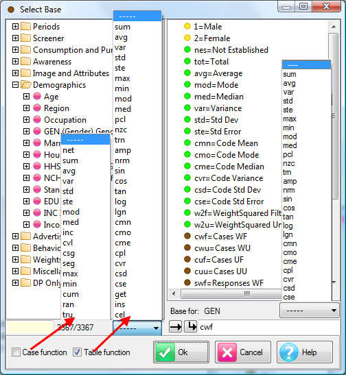
The left drop down (shown in both forms here) provides the Case and Table algebras as on the Table Specification form.
The right drop down provides the Codeframe algebra as on the Arithmetic form above.
This form is the only place where you can see all three levels of algebra because bases can be any expression whatsoever.
Some examples:
cwf
tot
#(c1+c2+c3)/3
@age(1/3)
@get#BrXClaimed(#c2/c1*cwf)
Exercise: Changing the Percentaging Base
As well as any of the standard base types, you can specify anything at all to be the percentaging base.
You can base on any vector in the codeframe, any of the standard statistics vectors, any expression on the vectors, any expression on the items of other code frames, on a set of inserted constants, and even on a vector from another table altogether.
This is done with the Local Base menu item on the Specification form.
Start a New table
Drag Occupation to the Top
Right-click on Occupation and select Base First
Drag Gender to the Side
Right-click on Gender and select Local Base
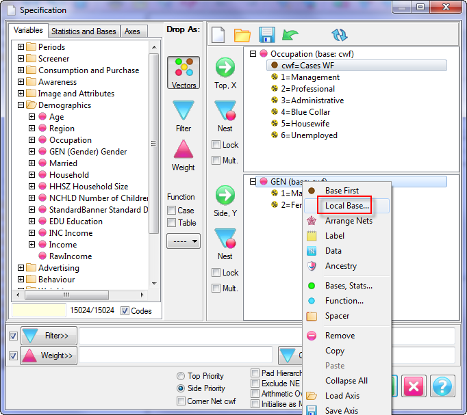
This opens the Select Base form.
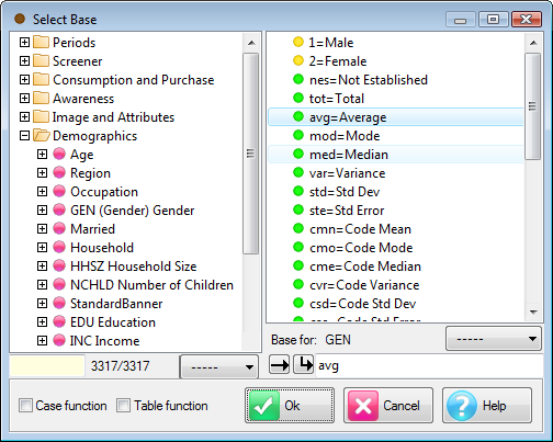
Double-click the Average node, as above, so that avg appears in the bottom right edit field (or type it in, or select and then click the bent arrow button).
This edit field is where the base expression is built up.
Click OK
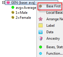
Notice that Gender is now indicated as having base avg. This applies for this specification only. Gender's default base has not changed from cwf.
Right-click on Gender and select Base First
Notice avg=Average is inserted at this time.
Click Run
When the table appears, set the toggles for Frequencies and Percents
Set Statistics to 1 decimal place in Properties|Cells
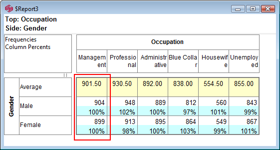
Notice the base for Occupation(Management) = 901.5 = (904+899)/2, the Gender average.
The percentages in this table now show the extent to which gender for each occupation differs from the average.
Note that these percentages are not in fact very realistic because the Demo job comprises mostly randomly generated example data only.
Headcounts and Multi-Response
For multi-response variables, sometimes the percentages are of the number of respondents (cases) and sometimes they are the number of responses.
The table Count by UBA filtered to Case(1) with Priority on the Side is:

The value at the base/base intersection can be either the sum of the top base values, here 1, or the sum of the side base values, here 1+1+1=3.
To have a 1 in the top left corner instead, set Priority at Intersections to Top.
The table becomes:
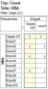
Ruby tables are completely symmetrical, so no assumptions are made about the orientation of a table.
Taking the base/base intersection as the sum of bases makes table interpretation across the 14 standard base types and the infinity of custom bases uniform.
If you have multi-response variables both ways, and want the headcount net in the top left corner for percentaging purposes, then use Count with either or both of cwf and code 1 as the first column.
For example, the table UBAN by UAAN with top priority is
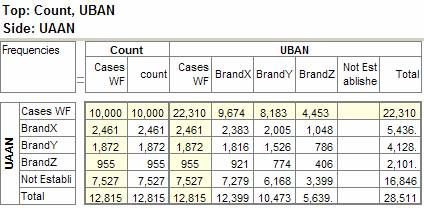
22,310 = 9674+8183+4453
With side priority, the table is
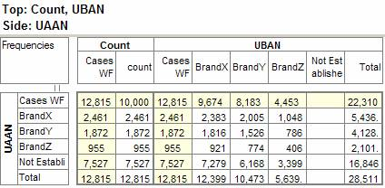
12,815 = 2461+1872+955+7527
But whether priority is top or side, the column for Count(1) remains the headcount, which is 10,000.
A corner base of 10,000 can also be achieved by checking Corner Net Respondents - see Priority at Intersections above.
This is all designed to give maximum flexibility, so that percentages of anything in any way can be achieved, such as for the Stacked table of Claimed Recall which has a row from a completely different crosstab as the base, specified like this:
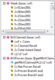
Statistics and Bases Tab
Standard Statistics and Bases are under the second tab on the left side of the form.
You can drag a statistic or base (like Total in the picture below) but it must land on some part of the variable, including any of its codes.
Bases always default to appearing before codes and statistics always default to appearing after the codes, but both can then be rearranged in any order.
You can select a statistic and click the Side/Top button.
If there is no selection in the Top/Side panel the statistic will go to the first item but this will only work if the first item is a codeframe.
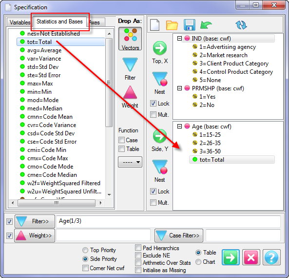
Show Statistics Vectors
Any of the standard statistic vectors can be dropped on any variable in the Top or Side specification trees.
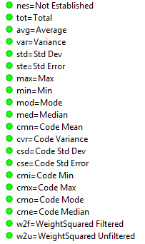
If you want the vector to respond to the Percent buttons on the ribbon, for example for Totals or Not Established, then toggle the % in the specification node.
By default, bases insert at the top, and statistics and Not Established insert at the bottom, but you can move any node to any position by drag and drop or use of the Ctrl-arrow keys.
The only exception to this is the percentaging base. It must appear first if you want it to take the base background colour and font.
Setting default drop bases and stats
Any of the items in the Bases/Statistics tree can be set as a default for top or side by a double-click.
Start a New table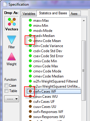
Select the Statistics and Bases tab
Bring cmn into view in the Stats/Bases panel and double-click on it
Locate cwf and double-click it three times
The horizontal mark indicates cmn is set as a default for drop operations on the side (row), the vertical mark indicates cwf is set as a default for drops on the top (column).
The cycle of symbols is
 (row)
(row)  (both)
  (column)
  (neither)
Drag Region and Gender to the Top
Drag Household to the Side
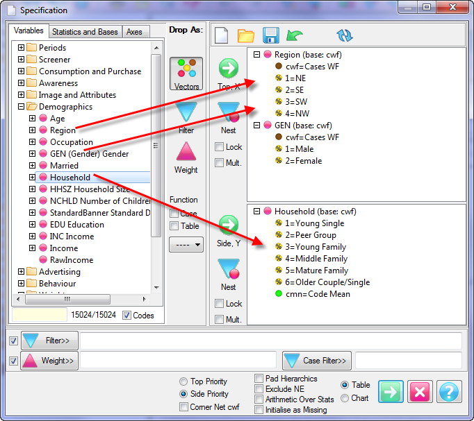
Note how the top variables come with cwf (saving you the trouble of selecting Base First) and the side with cmn.
A common set of defaults for table work would be cwf, nes and tot.
Back in the Statistics and Bases panel double-click again to cycle through the states to unset a default vector
The default statistics and bases are saved to job.ini
Axes Tab
Axes are any collection of things on the top or side, including any number of variables with bases, filters, weights, spacers, and so on.
The Specification form has an additional tab to hold prepared axes. This makes a few new things possible, for example:
Attaching the right filter and weight to variables that need them
Always having the right stats and bases where needed
Preparing banners and nets without constructing
The idea is that the analyst can build specs with axes from the Axes tree that are safe and simple to use.
You can create axes yourself, and DP may have prepared some for you.
You can drag any axis or folder to either top or side.
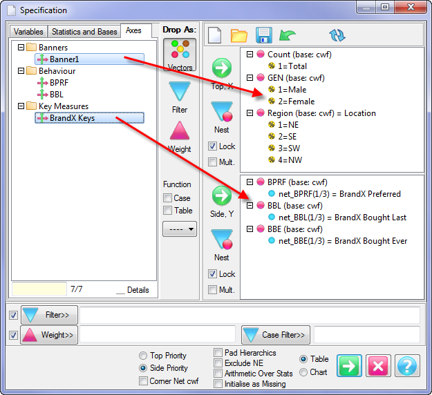
Using Axes
The picture shows Banner1 dragged to the top - several variables including some Presentation text; and BrandX Keys dragged to the side - several netted key measures.
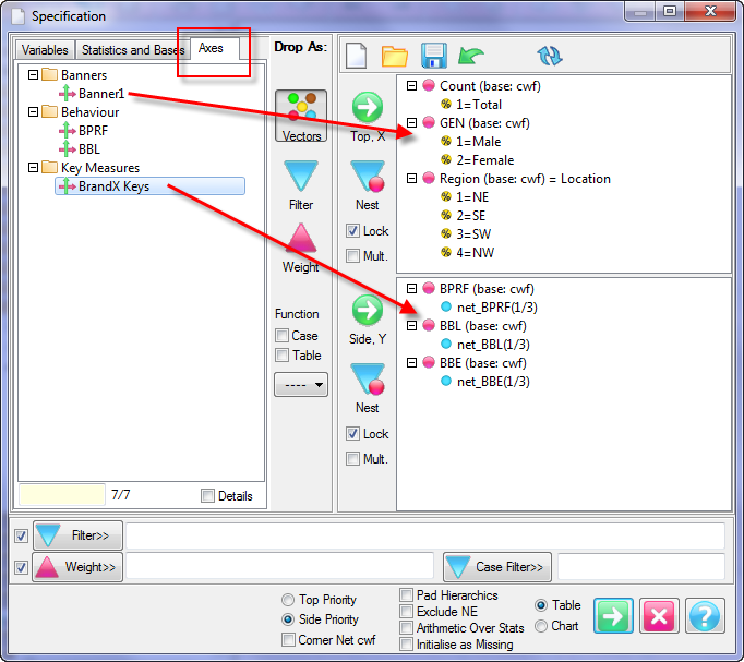
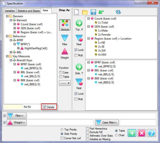
Click on Details to see the composition of the axes available - you can't delete or reorganise while in Details mode.
Creating Axes
The simplest way to make an axis is drag it from top/side to the Axes tab.
This will invite you to save the axis under a name and add it to the tree, if it is not there yet.
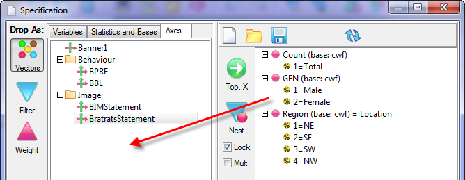
Drag any part of the axis to save the complete axis and add it to the tree.
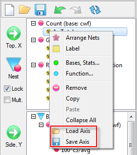
There are two menu items on the top/side right-mouse menu you can use also:
Load Axis opens a named saved axis (not necessarily in the tree).
Save Axis saves under a specified name and adds the axis to the tree.
Axes Tree Operations
You can rearrange the tree by dragging and using CTRL-Arrow keys.
You will be prompted to save the tree if necessary when the form closes or you can save it explicitly from a menu.
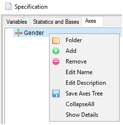
The right-mouse menu on the Axes tree includes:
Folder - make a new folder
Add - add a saved axis
Remove - remove an item
Edit Name - displays an edit prompt for the new name (You can also edit Folder names the usual way with the second mouse click, slower than a double-click.)
Edit Description - displays an edit prompt for the new description
Save Axes Tree - save any changes
Show Details - same as the Details switch
Delete nodes with the Remove item or [Delete] key (only when Details is OFF).
When you have Details ON the familiar Data/Ancestry items are visible for variables - and you can't delete or reorganise the tree.
When you close the specification form you will be prompted to save the axes tree if any changes have been made.
Axes Files
The files behind the scenes are:
The axes tree Axes.atr that functions in much the same way as the Vartree.
Axes.atr is loaded with the job and included in zips with the Vartree
It just contains the list of names of axes organised under folders
The variable tree Vartree.vtr
This is edited in the Edit Vartree form (DP only)
The Axes tree is edited directly on the Specification form.
Several “.axs” files in the Specs folder contain the details of each axis.
These can be loaded and saved directly on the Top/Side axes.
The tree is saved to the job folder C:RubyJobsDemo
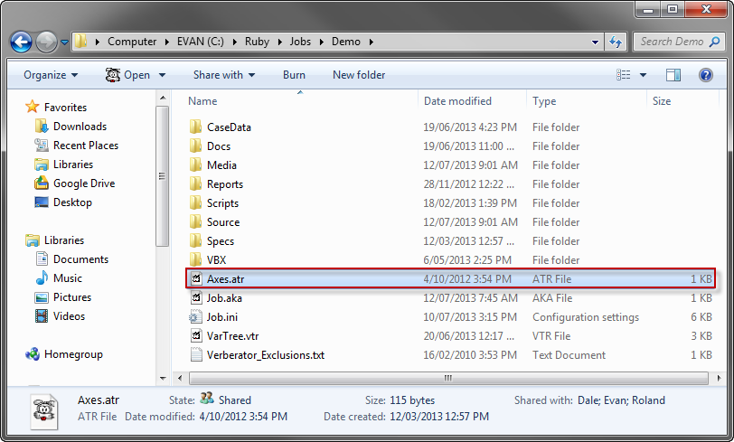
The axes defiinitions are saved to the Specs folder C:RubyJobsDemoSpecs
Banner1.axs
BrandX Keys.axs
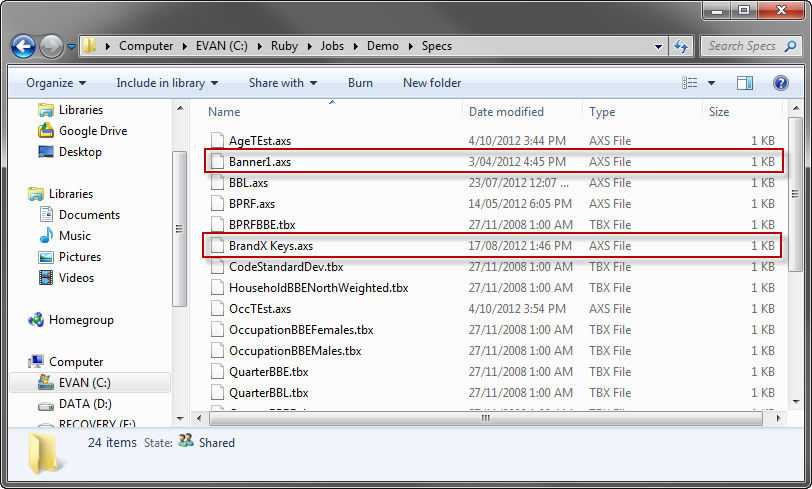
In RAM Form
 (Ctrl+M)
 The In RAM command on the Home tab of the Ribbon opens the In RAM form.
The In RAM form shows all reports in memory regardless of whether or not they are in open windows.
On closing a window, the data is not removed from memory, because often it will be needed again. This is especially true of the raw crosstabs used to assemble displayed tables and charts. Raw crosstabs are never redundantly regenerated.
The first tab shows all display tables in memory:
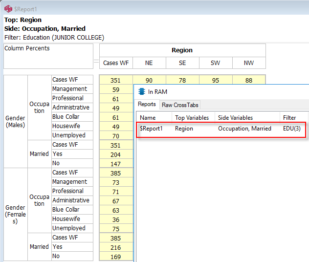
Here, there is only one, not yet saved, so named $Report1. The specification is Region by Occupation, Married, filtered to gender, all filtered to Junior College, so we expect four raw crosstabs:
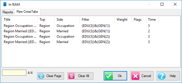
The second tab shows the raw crosstabs needed to populate the cells in display tables and charts. The Flags column is the Runtime flags from the Specification form and the Time column records the generation time in centi-seconds.
You can remove all raw crosstabs and regenerate the report. If you remove the report, but keep the raws, then respecify and rerun the report, it will generate almost instantly because the raw cross tabs are still in RAM. This also means that specification axes can be re-arranged without costing a regeneration.
Clearing Memory
 Clear Page clears whichever tab you are on.
 On clicking Clear All every table and chart in memory will be cleared and every window closed with no prompt to save.
Clearing the Raw CrossTabs list does not close any windows or remove any reports from memory.
This is useful for retrieving memory.
The raw crosstabs can be restored by respecifying and rerunning the report.
Raw crosstabs are necessary if changing the top/side priority or running significance tests.
Selecting
If you double-click on any report or select one and click OK, the In RAM form closes and that report is displayed.
Raw crosstabs appear in a text window.
To examine a raw crosstab, highlight/copy/paste (use Control/Insert key combination) into a spreadsheet.
Export Group
Copy

Opens the Clip form.
Send To

Send To is used to export reports to MS Office applications. See Send To any MS Office and Send to Excel.
See also Exporting Reports in Concepts and Definitions
Clipping
The Copy to Clipboard button in the Export group on the Home tab opens the Clip form: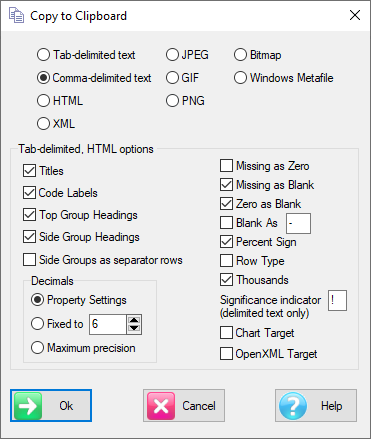
This sends the current report to the clipboard as either text or a graphic.
The various graphic types have different advantages in different circumstances:
The HTML clip is an HTML version of the table as drawn and will paste directly into Excel.
The XML clip is a proprietary Ruby Report format that is easily interpreted.
The delimited and HTML data switches offer some pre-formatting:
Titles: Include the Top, Side, Filter, Weight information at the top.
Code Labels: Include code labels.
Top Group Headings: Include group headings as part of the top code labels.
Side Group Headings: Include group headings as part of the side code labels.
Group Headings as separator rows: Include group headings on the side as extra rows separating blocks of data.
Decimals: Property Settings means use the decimal settings on the Properties|Cells tab. Fixed to exports all values with the decimal places fixed to the value in the thumbwheel. Maximum precision exports values with as many decimals as needed up to 15 digit precision - trailing zeroes and decimal points are removed if possible.
Missing as Zero: Replace missing values with zeroes
Missing as Blank: Copy missing values as blank rather than “*”
Zero as Blank: Replace zero values with blanks
Blank as : Flag all blank cells with the specified character - the default is a dash
Percent Sign: Includes percent signs for percentaged data.
Row Type: Add col% or row% to percentaged labels if there is a need to distinguish rows.
Thousands: Format numbers with thousand separators.
Significance indicator: Indicate significance test results by appending one, two or three of the character after the number. For example 12.4!! was significant at the second level. This only applies as a substitute for colour distinction where colour is not available. The HTML clip uses colour instead and the Group tests have an extra row/coloumn to show ABC etc.
Chart Target: Don't send text that won't chart. This prevents the !!! suffix and ABC rows/columns that indicate significance from appearing in the sheet behind MSChart objects.
OpenXML Target: An internal format which is the input to the conversion to OpenXML (that is, to the Excel XLSX format). This is generally useful for any circumstance where you need all properties and cell data in the same place for your own custom conversions to other software formats.
Clipping Examples
Here are some examples of pasting exports straight into Excel with various switch settings.
Using this table:
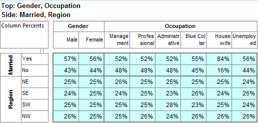
Titles, Code Labels, no Group Labels.
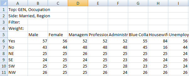
Titles, Code Labels and Group Headings as separate rows.
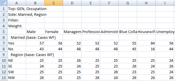
as HTML
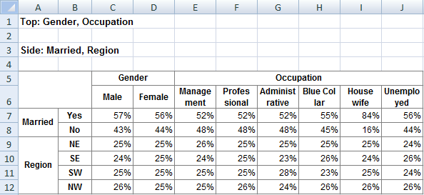
Send to any MS Office
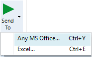
Opens the Exports form:
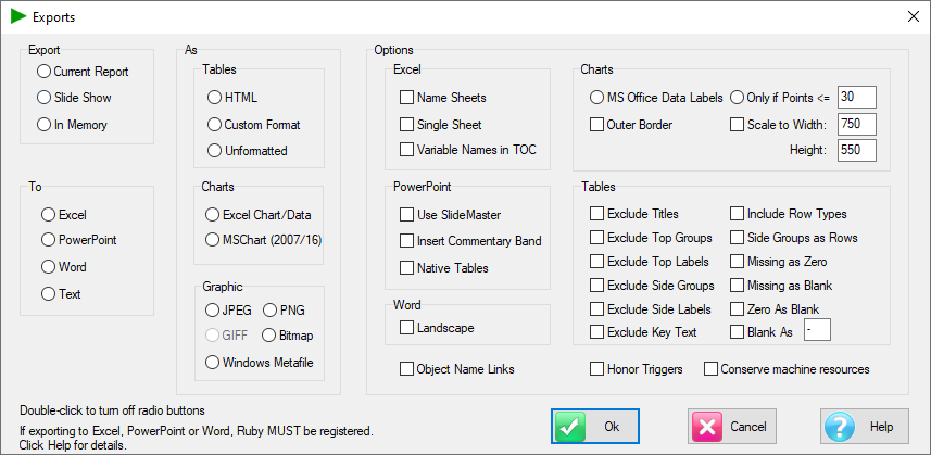
Use this form to control exports to MS Office applications. This is a much more sophisticated process than a simple copy/paste because as much cosmetic and layout information as possible is transferred. What you see in Ruby is, as far as possible, what you get in your selected destination application.
Export
Specifies what to export - just the current report, all reports in the current slide show or all reports in memory. In Memory does not just mean all open windows. You may need to check the In RAM form first to see what will be delivered.
To
Select the target MS Office application or Text to export to a text file.
As
Tables and Charts will look as close to their Ruby source as possible including colours, fonts, label nesting, chart type, horizontal bars etc.
Data transfers are done by HTML copy/paste for Tables|HTML and for Charts|Excel Chart/Data and Charts|MSChart2007/13.
Tables|Custom Format uses tab-delimited, and then independently formats each table cell. This is very accurate, but also very slow. If you require a custom format (to enforce house or client standards), then examine and edit the CustomFormat() function in Exports.js accordingly.
Tables|HTML misses some original properties, such as displayed decimal places for percentages (copy to Excel enforces either 0 or 2 DPs), but exports are dramatically faster. If you need other than no or 2 decimal places for percents then use Send to | Excel.
For charts, Excel Chart/Data means that an Excel workbook will be inserted into Word or PowerPoint. This will increase the file size, so should only be done if you really need access to Excel functionality in the target document. The workbook will have two sheets - one for data, and one for the chart. These export settings...
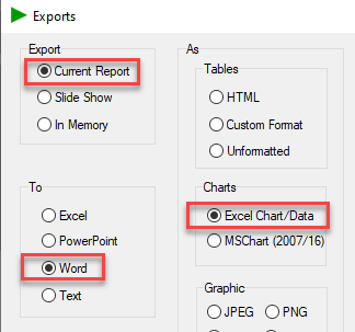
...deliver to Word as an Excel object, which appears like this on a double-click:
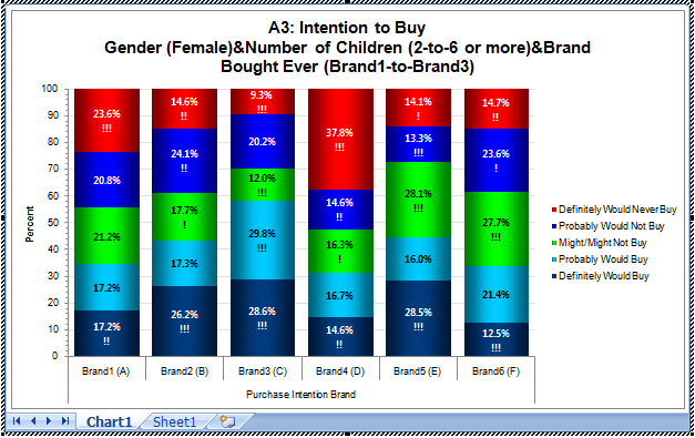
The chart is duplicated by Office on Sheet1. Remove it to see the data source table. Unless you need Excel functionality (such as calculating additional columns or rows), the MSOffice (2007/2016) option is usually the best for Word or PowerPoint.
Enable Object Names
Checking Object Names assigns the Ruby report name to the corresponding PowerPoint object. This makes it possible to keep a connection between the Ruby report and the PowerPoint object for updating or other purposes. Note that due to a limitation in PowerPoint, object names cannot exceed 32 characters.
MS Office Data Labels lets PowerPoint handle all the data labels (instead of following the Ruby chart properties). To prevent unreadable clutter on long series, an upper limit on the number of points can be set.
Outer Border puts a thin black border around the chart.
Scale To scales the Ruby chart to the specified width and height (in pixels). If you want font sizes to stay the same, then set the fonts at the scale you intend to export at. The current window's scale is indicated at the bottom left as you drag an edge.
Honor Triggers looks for text fragments in the report names which 'trigger' and custom behaviour you may have built into Exports.js (there are several examples - search Exports.js for 'trigger').
Use PPSlideMaster will look for a copy of PPSlideMaster.pptx in the Job directory (the directory which contains job.ini and vartree.vtr for this job). The slide master can be anything you like. The one supplied in RubyJobsDemo uses the Red Centre colour-scheme and logo. You can modify this in any way, or supply a completely new one, but the name PPSlideMaster.pptx is expected, and so should be retained unless you have modified Exports.js accordingly. The footer and other details of the Slide Master are often manually changed for each job and/or update - hence each job needs its own version.
The Exclude Groups switches are for when the nesting and parent variable information is not wanted.
Insert Commentary Band inserts a custom text box underneath the title region:
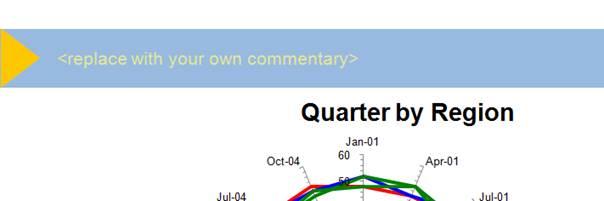
For details see the document Ruby Push Pull Reference Manual.pdf on the Ribbon Help page.
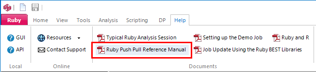
Send To Excel
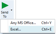
Opens the Ruby to Excel form, which calls the stand-alone executable RubyToExcel.exe. The Ruby table and chart formatting is preserved as far as possible.
RubyToExcel.exe is a much faster alternative to the internal Ruby export mechanism. It can handle huge tables (>1,000,000 cells) and does not require Excel itself if invoked with command line arguments.
The export creates a native Excel file. If Excel is installed and the invocation is manually from the Ribbon Home page then the Excel file opens automatically.
RubyToExcel.exe is stored in the same folder as Ruby.exe.
Ruby must be open and, for manual invocation, either a single report or a slideshow must be active.
There is an extensive set of command line arguments for batch processing.
RubyToExcel opens with these defaults:
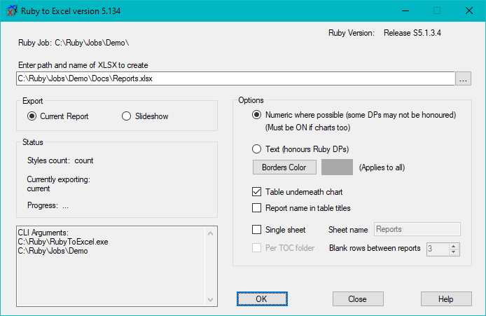
Ruby Job: The job Ruby currently has open
Ruby Version: The Ruby version being accessed
Enter path and name of XLSX to create: The Excel file to write
Export
Current Report: Export the single report with focus
Slideshow: Export the selected TOC slideshow
Options
Numeric: Export as numeric - allows average, sum, count by cell drag in Excel. Numeric must be ON if a chart, or if the slideshow contains charts (cannot plot a string)
Text: Export all cells as text - overrides by text matching for decimal places will be honoured
Borders Color: Set the border and gridline colour for all reports
Table underneath chart: Places the data source table for the chart underneath the chart - if off then the table's top left cell will be the same as the chart top left, which can be useful if small tables and you want to see only the chart
Report name in table titles: Export the report name as shown in the TOC as the first title item
Single sheet: Send all reports to a single spreadsheet, rather than one sheet per report
Sheet name: The name of the single sheet
Blank rows between reports: The number of blank rows to insert between each table in the single sheet
PerTOCFolder: Create a new sheet for each child folder in the selected slideshow, where the sheet name follows the child folder name
Status
Styles count: The number of unique Excel cell styles required (all combinations of fonts, borders, format, alignment etc) - this is primarily a diagnostic
Currently exporting: The report currently being exported
Progress: Shows the major steps - saving may take a while on large exports
CLI
Echoes the command line arguments if RubyToExcel is invoked from a script or batch file - see below for details
OK
Run the export
Close
Close the form
Help
Open a local Help form on the latest RubyToExcel functionality
Once OK has been clicked, each of the Ruby reports will briefly display and then a confirmation message will indicate that the file has been saved.
Excel will then open, showing a menu of hyperlinks to and the specification details of each report:
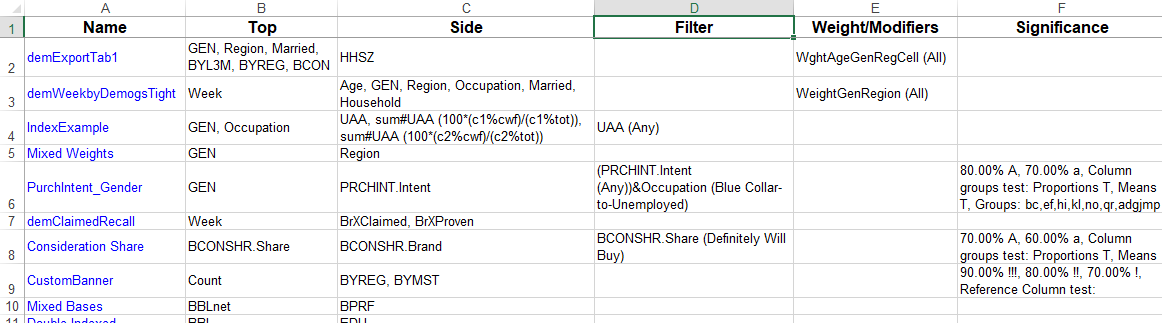
Batch Processing and CLI Arguments
For automated processing you can call RubyToExcel with command line arguments. The arguments are
Arguments can be invoked in several ways:
1. Create your own desktop shortcut to RubyToExcel.exe, and then set the CLI arguments as the target property
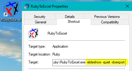
You would do this if you always wanted to run with the same arguments for all or most jobs.
2. Create a system batch file (*.bat) which calls RubyToExcel with the required arguments, and then execute the batch from a command console
For example, create the file RubyToExcelBat.bat in a text editor and save to the job folder:
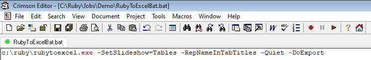
Then run from the console as
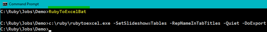
Note that any argument with spaces must be quoted, eg
c: uby ubytoexcel.exe '-SetSlideshow=Standard Tables' - DoExport
3. Call from a script
This is the best approach for automating an entire job - update, process, then export, all from the VSX project.
There are many examples at RubyJobsDemoVSXCallRubyToExcel.vb.
Note that the argument string must itself be quoted, so arguments with spaces need double quoting, eg
cli = ' ''-Workbook=My Batch Test'' -RepNameInTabTitles -RowsGap=4 -DoExport -Quiet '
The commented examples are
'' Export current slideshow (set from the GUI) to Reports.xlsx (being the default name) as one report per sheet, open in Excel, no overwrite prompt
cli = '-SlideShow -Quiet -DoExport'
'' As above, but do not open in Excel
cli = '-SlideShow -DontOpenFile -Quiet -DoExport'
'' As above, but insert the report name before the other titles, save as ReportBook.xlsx and open in Excel
cli = '-SlideShow -Workbook=ReportBook -RepNameInTabTitles -Quiet -DoExport'
'' All reports to a single sheet named Reports (the default), with two blank rows to separate, report names, save to My Report Book.xlsx
'' Note double double quotes - needed because the -Workbook argument has spaces
cli = '-SlideShow -SingleSheet -RowsGap=2 ''-Workbook=My Report Book'' -RepNameInTabTitles -Quiet -DoExport'
'' As above, but with named sheet too
cli = '-SlideShow -SingleSheet -RowsGap=2 ''-Workbook=My Report Book'' ''-Worksheet=My Work Sheet'' -RepNameInTabTitles -Quiet -DoExport'
'' Follow the first level of child folders under the slideshow parent folder, exporting each folder to its own worksheet
cli = '-SlideShow -PerTOCFolder -RepNameInTabTitles -Quiet -DoExport'
'' As above. but set the slideshow by citing the parent TOC folder
cli = '''-SetSlideshow=Standard Tables'' -PerTOCFolder -RepNameInTabTitles -Quiet -DoExport'
'' Test three arbitrary batched folders
cli = ' ''-Workbook=My Batch Test'' -RepNameInTabTitles -RowsGap=4 -DoExport -Quiet '
cli &= ' ''-Batch=Standard Tables/Demographics,Demogs;Standard Tables/Advertising Awareness,AdAwa;Tables,Tables'' '
'' Same three batched folders, but specified by line for readability (there could be a lot of folders)
cli = ' ''-Workbook=My Batch Test'' -RepNameInTabTitles -RowsGap=4 -DoExport -Quiet '
cli &= ' ''-Batch=Standard Tables/Demographics,Demogs;'
cli &= 'Standard Tables/Advertising Awareness,AdAwa;'
cli &= 'Tables,Tables'' '
Known Limitations and Issues version 5.135
1. If a table has Percents as Proportions ON, there is a base column, and there are column percents, then the exported base column proportions format with frequencies decimal places. For example, with frequencies at DP0 and percents at DP2
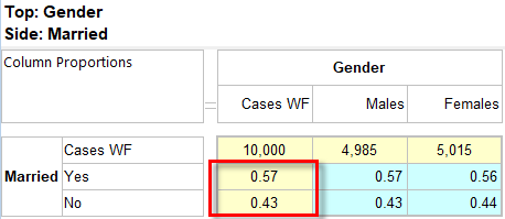
the export is the correct value (0.57) but formatted as DP0.
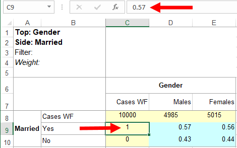
The work-around is to set Frequency DPs to the same as Percents:
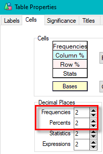
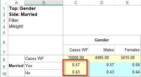
2. If the last row is a complete variable block
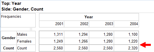
the top border is lost:
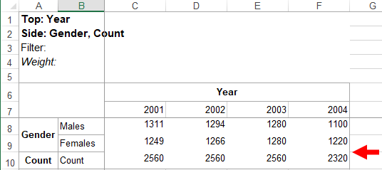
3. If a chart's category axis items have been restricted by raising the start index or lowering the end index
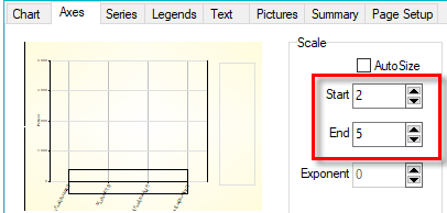
then if a flat axis you will get a warning
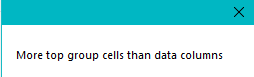
and if a nested axis, an error
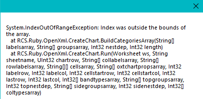
The work-around is to reduce the category items in the report specification to only the ones you want charted.
4. In MSChart cluster bars cannot straddle both Y1 and Y2. This chart, with Males on Y1 and NE (north east) on Y2
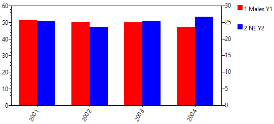
exports as overlapping bars.
Un/Redo Group
When there is something to undo, the Undo button on the Home tab of the Ribbon becomes active. Clicking on it undoes the last change, and clicking on the Redo button redoes the last Undo.
For more information, see
Undo, Redo on Tables
Undo, Redo on Charts
Filters Group
The Drill and Switch dropdown menus are set up by DP in the Edit Custom Menus form.
The Last item, 'Select', opens the Build Expression form where you can define any other filter when you need more than the presets.
Any applied filters can be removed or added back in by using the Undo/Redo buttons
.Drill Down
The Drill Filter combines subsequent selections with & = AND. For example, Gen(1)&Married(2)&Region(3) specifies single male from the southwest region.
Switch To
The Switch Filter replaces the existing filter with whatever selection is made.
Properties Group
Active

Opens the Properties form appropriate to the type (table, chart, map or gauge) of the active report:
Table Properties
Chart Properties
Perceptual Map Properties
Gauges Properties
Common

Opens the The Common Properties form which has four tabs from the Table Properties form relating to underlying data properties which are common to tables and charts:
Significance
Flags
Sort
Hide
Vectors
Callouts

Opens the Chart Callouts form.
Table Properties
The Table Properties form organises almost every setting that can change the way a particular table appears.
There are a couple of session-wide settings on the Preferences form (show priority/sort indicators, spreadsheet style buttons) but everything else is here.
You cannot change the underlying data - that can only be done in the Table Specifications form - but you can change how it is treated in the Vectors tab by applying rolls etc.
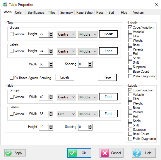
Table-specific tabs
Labels: change cosmetics for row/column labels.
Cells: change cosmetics for table cells and the key area.
Titles: change cosmetics for titles.
Summary: change cosmetics for the optional summary table.
Page Setup: settings for printing with headers and footers.
Common (Table & Chart) tabs
Significance: apply inbuilt or scripted significance tests.
Flags: frequency/percent flags, date format, force zero values to be missing, percents as proportions, corner priority.
Sort: settings for sorting rows and columns.
Hide: settings for hiding rows or columns by various criteria.
Vectors: details of each row and column including roll, suppression, scale, shift.
Table Window Areas
The areas in a table window are described as:
Top and Side Groups
Top and Side Labels
Central Cell Area
Key Area
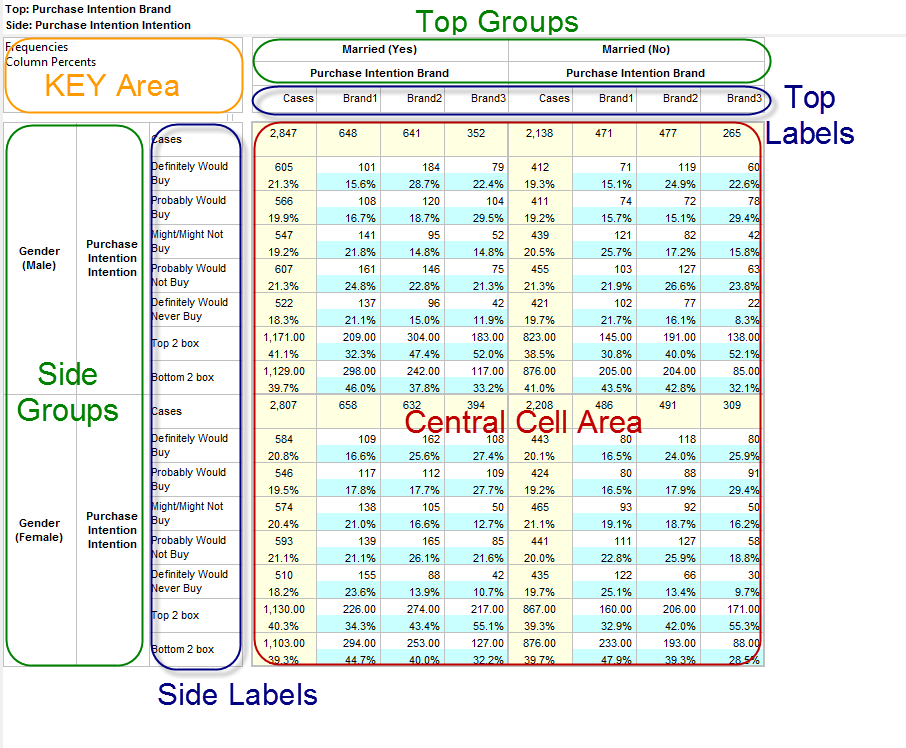
Labels tab
The Labels tab has similar sections for the Top and Side label areas, each containing text settings for Groups and Labels.
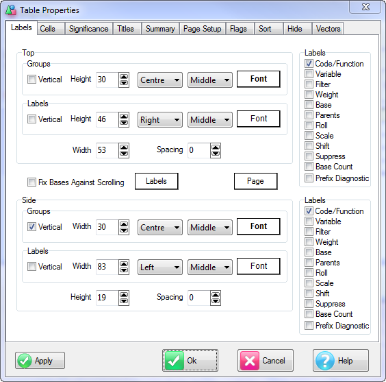
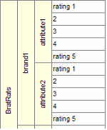
Groups means the top or left most lines of the area where you see variable names, filters, weights and other grouping information (pale yellow here); Labels has a specific meaning here referring to the inside row or column labels (white).
Vertical: Text can be vertical or horizontal.
Height/Width: Height of top lines, width of side lines.
Alignment: Text can be horizontally aligned left, right or centre.
Anchor: Text can be vertically anchored top, bottom or middle.
Font: Select any font and colour.
There are two additional controls inside the Top and Side boxes:
Width/Height: Width of top columns, height of side rows. This is effectively the cell width and height.
Spacing: This is the amount of spare space that will be forced - see below.
Other settings in between the top and side boxes:
Labels: Background colour for label and key areas.
Page: Background colour for the rest of the window outside the four areas.
Fix Bases Against Scrolling: As you scroll the table, keep base rows and columns at the left and top.
Finally, the set of Labels switches on the right determines how the row/column labels will be built up from information available. Generally the code label will be all you need but if you have the same row differently rolled or based, or the same statistic such as code mean differently filtered, you might want to see that; if the data is scaled, shifted or suppressed you would probably want that in the label as an aid to interpretation and understanding.
Code/Function: the normal code label or function expression.
Variable: the parent variable of the code. In tables this is obvious from the group structure but is often useful for chart legends or axes.
Filter: any local filter applied to this vector.
Weight: any local weight applied to this vector.
Base: the base used for percentaging (if topmost row or leftmost column in a variable block).
Parents: for hierarchic variables, the parent path of the specification tree.
Roll: any roll applied to this vector.
Scale: scale factor for this vector.
Shift: translation for this vector.
Suppress: points suppressed at the start or after missing values.
Base Counts: adding n= base counts to labels. 'n' is the Base Count Tag set on Preferences|Job Settings.
Prefix Diagnostics: the label will have the diagnostic form in square brackets before the longer forms - e.g. [Gen(1)] Male
Spacing Settings
Where text sits inside a text box is determined by the spacing settings on the Labels tab, and the Text Gap from Edge setting on the Cells tab.
Text Gap from Edge is an inside margin which ensures there will be that much white space before the edge in any direction.
Spacing depends on top/side, alignment and anchor settings.
For the Top labels area the spacing is to the left, right or both sides of the text depending on alignment.
For the Side labels area the spacing is above or below the text depending on anchor.
For left-aligned text space is forced on the left; for top-anchored text space is forced on the top; for centre-aligned text space is forced on both sides, etc.
This is useful for forcing space between the vector labels.
For example, these settings...
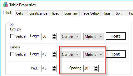
...appear as:
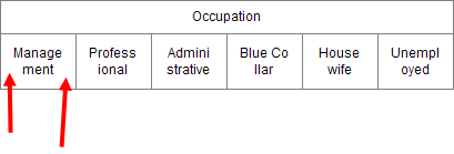
Cells tab
The Cells tab has settings for the colours, fonts and contents in the cell and key areas, grid lines and general gaps between text and borders.
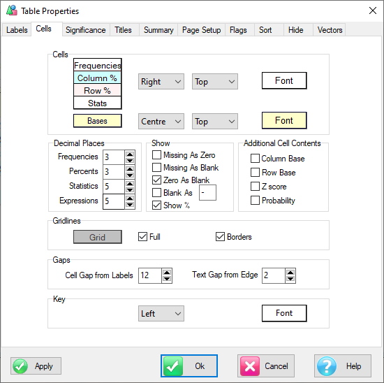
Cells
Frequencies: Colour behind Frequency numbers in cells and the key area.
Column%: Colour behind Column Percent numbers in cells.
Row%: Colour behind Row Percent numbers in cells.
Stats: Colour behind significance letters and other statistical information in cells.
Alignment: Left, right, centre alignment for cells except bases.
Anchor: Top, middle, bottom anchor for cells except bases.
Font: The font for all cells except those in a percentaging base row or column.
Bases: Colour behind Base numbers.
Decimal Places
Independent decimal places for frequencies, percents and statistics and expressions.
If the Preferences switch is ON then any expression that contains AVG or CMN is recognised as a Mean for the purpose of decimals and will use Statistics decimals rather than Expressions decimals.
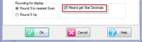
Missing as Zero: If a cell value is missing (*) then show a zero.
Missing as Blank: Do not show missing as *
Zero As Blank: Do not show zeroes
Blank As : If either missing or zero cells have been set to show as blank, the blank cells can be flagged with the specified character.
These settings cascade, so you could have missing->zero, zero->blank, blank-> character
Show %: Turn the % sign ON or OFF for percentages
Additional Cell Contents
Show the column and row base values, the Z or T score depending on the statistical test, and the probability of there being a significant difference.
Gridlines
Gridlines are one colour, generally one pixel thick, with a thicker line separating major blocks.
Colour: Colour to use for all grid lines
Full: Show thin grid lines separating all rows and columns.
Border: Show thicker grid lines separating major blocks - i.e. between cells in the outermost group line and around the entire cell area.
Gaps
Cell Gap from Labels: This is the small gap between the labels and cell areas where you may see sort indicators and alpha labelling of columns for significance testing.
Text Gap from Edge: The number of pixels to keep between a text item (everything except titles) and the nearest border.
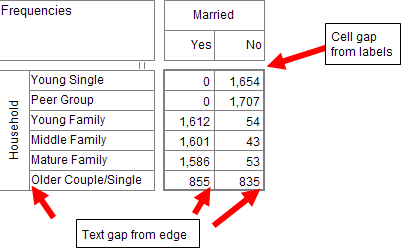
Key
Alignment: Left, right, centre alignment for text in the key box (top left of table).
Font: Font for text in the key box.
Significance tab
This has the settings for significance testing.
There are several in-built significance tests or you can attach an external Java or VB script to perform any testing you like.
See Statistical Significance for an overview.
See Appendix 8 - Statistics in Ruby for the mathematical definitions of the statistics tests.
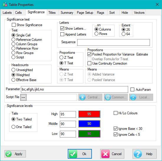
Show Significance: This matches the Show Significance toggle
 in the Display Status Group on the Home tab of the Ribbon.
Letters: Labels columns or rows with letters of the alphabet so they can be identified for group significance tests.
The letters can be on columns or rows, 26 upper case for two levels of significance (lower case indicates lower significance) or 64 characters as abc...zABC...Z1234567890-= for a single significance level.
Sequence: Indicate a custom sequence of letters using dots or spaces for blanks - e.g. .A..BCD. This allows the 64 testable vectors to be spread out over an axis with more than 64 vectors.
Test: The in-built tests are described in Appendix 8 - Statistics in Ruby.
Depending on the test you can choose Z or T tests independently for Proportions and Means.
The default settings are the most common ones.
HeadCounts: what to use for n in degrees of freedom and variance estimates.
Proportions/Means: choose T or Z test together with the appropriate settings for estimating variance.
Parameter: This is used by the group tests to indicate which columns or rows to test.
e.g. For the Column Groups test, “ABC,EFG” means test columns ABC against each other and columns EFG against each other.
If the field is blank it means all columns or rows. Scripts can also retrieve this text.
AutoParam: If checked, then determine the groups from the axis variable boundaries.
Script File: Customised significance testing in Ruby is done with external scripts. The file is specified here.
If it is in the Jobs folder it will have a leading '@' character, if in the Ruby folder a leading * character, and if in the job's Scripts directory just the file name. The script cannot be in any other location. Append Letters, Sequence, Parameter and the High/Middle/Low thresholds can be retrieved by a script, so that the same script can be applied to different tables. All other settings are disabled to the user, and will be set appropriately by the script. For examples see the files RubyJobs.js, eg PairSigTest.js.
Central: Browse for a script in the Ruby folder.
Common: Browse for a script in the Jobs folder.
Local: Browse for a script in the job's Scripts folder.
Tails: Set for one-tailed or two tailed tests.
Middle/High/Low: Sets the significance threshold levels and the font colours for the cell text (for tests that use colours).
A script can both retrieve and set these.
Hi/Lo Colours: For single cell tests, colours indicate above or below the significance threshold.
Ignore Base < 30: Don't test significance where base counts are less than thirty.
Ignore Cells < 5: Don't test significance where cell counts are less than five.
Titles tab
The Titles tab holds colour and font settings for the Titles area at the top of the table.
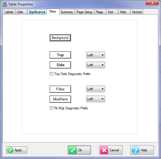
Background: Background colour.
Top: Font and alignment for text listing the top variables on the table.
Side: Font and alignment for text listing the side variables.
Top/Side Diagnostic Prefix: Insert the diagnostic form of the expression in square brackets before the longer forms.
Modifiers: Font and alignment for text describing weighting and sorting.
Filter: Font and alignment for text describing the overall filter.
Flt/Wgt Diagnostic Prefix: Insert the diagnostic form of the expression in square brackets before the longer forms.
The actual text that appears here is determined by the Label Mode setting on the System General tab of the Preferences form or more directly from the Display Status group on the Home page
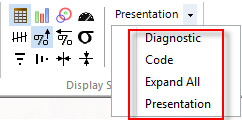
A Presentation title can be specified from the popup menu in the titles area that will replace all four individual text items with just one, using the Top font and alignment properties.
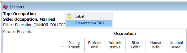
Summary tab
Every table can have a summary table attached as a floating window.
Specifying the calculations for the rows and columns is done in the Summary Planner.
The summary table's cosmetic settings are shown here.
This is almost identical to the similar tab on Chart Properties.
Page Setup tab
These are the print settings for hard copy if Override Batch Print Settings is ON.
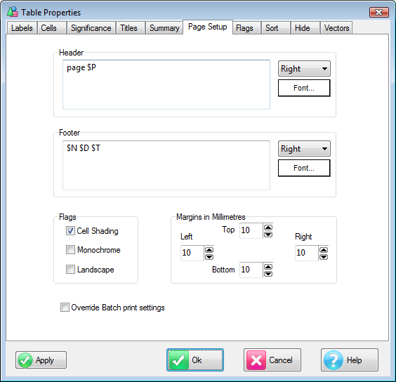
Header/Footer
This is the text that will appear as a header or footer on the printed page.
You can force white space by entering extra Returns and you can insert some dynamic information with substitution text.
$D for date
$T for time
$P for page number (for batch printing)
$N for file name.
You can set alignment and font for these as well.
Margins
Printers vary somewhat. If more spare selvedge space is needed, that can be set here.
Monochrome
This forces all fonts, lines and patterns to black, and the background and graph box to white.
Pictures are left alone because most printers handle grey scaling automatically.
Landscape
Usually charts are printed one to a page in landscape mode.
When printing batches of charts, if two charts in a row are set to Portrait (Landscape off) they will both be printed on the one page at half size.
Cell Shading
A separate color/monochrome setting for cells in particular.
You may want the table monochrome in general and yet still want different backgrounds for frequency and percent numbers.
Note that apart from Cell Shading, this is identical to the page setup tab on Chart Properties.
Override batch print settings
When batch-printing Ruby usually uses the settings from the Preferences form for the entire batch.
If you have a report with particular print requirements you can set this switch ON.
Flags tab
The Flag settings are common to both tables and charts.
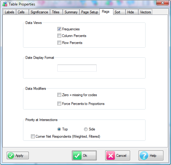
Data Views
These switches match the buttons
on the ribbon.Frequencies: Show frequency counts in cells.
Column Percents: Show cell values as percentages of the base values supplied by the Side specification.
Row Percents: Show cell values as percentages of the base values supplied by the Top specification.
Date Display Format
If your rows or columns are dates you can override the supplied labels with a date format.
This is similar to the Windows format settings using one, two or three letters to mean progressively more detailed text for day, month and year - with the addition of q meaning Quarter.
Any other text is copied verbatim.
For example,
“d mmm yy” shows as “3 Jun 08”
“start qq for yyyy” shows as “start Qtr3 for 2008”
This is useful for removing the day number or month number. It is used more often for charts than for tables.
Data Modifiers
Zero = missing for codes: Treats a zero cell value as if it were missing data.
This determines one feature of the rolling (moving average) algorithms.
When they encounter a missing value the smoothing process is suspended, starting up again when the next non-missing value is met.
This ensures that points with missing data remain missing.
Designating zero as missing therefore prevents zero values from pulling down rolled values.
If you need both zeroes and missing, then initialise the table as all missing in File|Preferences|Job settings.
Force Percents to Proportions: Showing row and column percents usually means frequency/base*100 but there are circumstances where the proportion may be preferred such as a table of the average number of brands recalled or bought or average price. If this switch is on, the *100 step is skipped leaving the result as a decimal with no % sign.
Priority at Intersections
There are some situations where cells may have ambiguous content.
When you have a row base and a column base, especially with multi-response and other complicated data, the cell where they intersect may find a different number in the row base and the column base.
This switch determines which number is displayed on the table.
This is indicated on the table window by an equals sign in the gap between the labels and the cells.
NB: These switches also appear on the Specification form for setting before running the table.
The other circumstance where a cell could be ambiguous is statistics intersections.
If there is a Code Mean column and a Total row, then the priority determines whether to show the total of the code means, or the code mean of the totals.
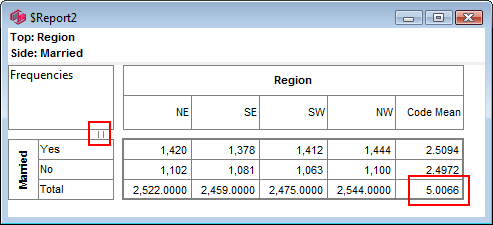
Side priority, so the bottom right intersection cell shows the total of the code means, 2.5094+2.4972=5.0066.
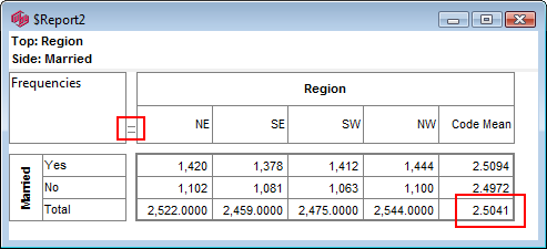
Top priority, so the bottom right intersection cell shows the code mean of the totals.
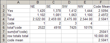
Verifying the calculation in Excel shows the final code mean 2.5041 calculated as 25041/10000.
If the priority switches are disabled then the table was loaded from file.
The reason they cannot be changed is because finding the other number that might go in an ambiguous intersection cell requires going back to the raw crosstabs that underlie the display table.
These are not part of the file load but can be generated by rerunning the table - select Specification from the popup menu and just click Run.
The Priority switches will now be active.
The Corner Net Respondents switch only affects the fixed base intersections. If you want the corner cell to always be Net Respondents set this switch ON. The Net value will then be used for percentaging bases and statistics that use the corner value (e.g. Single Cell).
Sort tab
These settings are common to both tables and charts.
Note the new Ungrouped and Band settings, introduced at Ruby version 5334. A change to old settings for some reports may be required - see the section Ungrouped Sorting below.
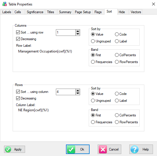
The Sort switches match the Sort Rows and Sort Columns buttons in the Display Status group on the Home tab of the Ribbon:
. The vector used as the sort key is indicated on the table window by a small circle in the gap between the labels and the cells.
Sort using row/column: for sort by value, identify the row to use when sorting columns and vice versa.
Decreasing: Sort in decreasing order, OFF for increasing. Since the high values are usually wanted at the top/left of a table, the default is Decreasing. These correspond to a right click on the Ribbon sort buttons
 .
.Row/Column Label: The rest of the space is for displaying the label (which could be quite long) of the sort row/column whose index number appears in the thumbwheel.
Sort by: sort by cell values, by the numeric code order in the variable's code frame, alphabetically by the axis labels, or ungrouped. A sort on Label or Code does not require an opposite key - the selected axis is sorted, unlike Value. For Ungrouped sorting, see the section Ungrouped Sorting below.
Band: The vector of values which controls the sort. Use First to sort on the first band (whatever that may be), Frequencies to sort on the frequency counts, ColPercents to sort on columns percents, or RowPercents to sort on row percents. The sort vector need not be visible in the table.
Codes can be flagged to be excluded from sorting in the Edit Variables form.
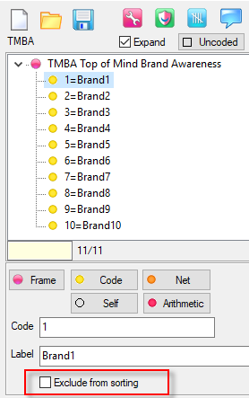
Ungrouped Sorting
Ungrouped means to sort across the variable boundaries. Individual rows or columns within a variable block are broken out into sorted order.
Previously, the only supported ungrouped sort was the special case where every row or column comprised a single band of the same type, for example
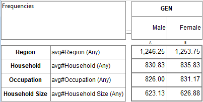
To achieve this sort order from version 5334 and later, set Ungrouped to ON:
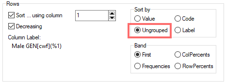
Consider an analytical requirement for a table of the highest demographic frequency count:
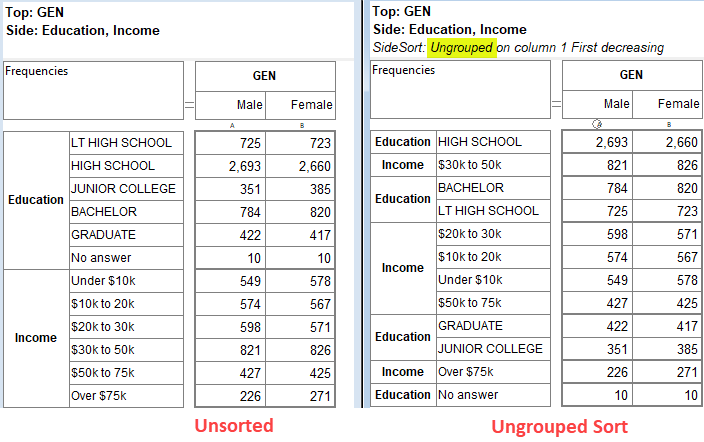
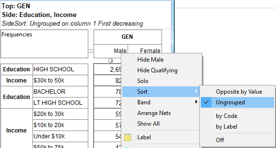
The rows have been sorted on column 1 regardless of the variable blocks.
The sort band is independent of the table display. The next table is sorted by row percents, using the Band context-menu item
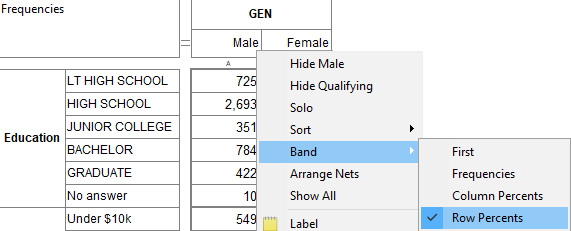
but displays frequencies only:
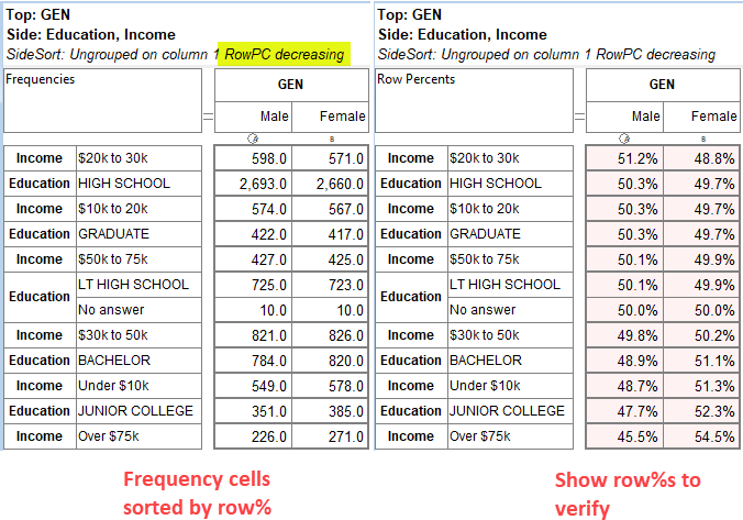
Band | First means the first displayed of frequencies, column% or row%. This is set as the default for all existing reports.
Hide tab
These settings are common to both tables and charts.
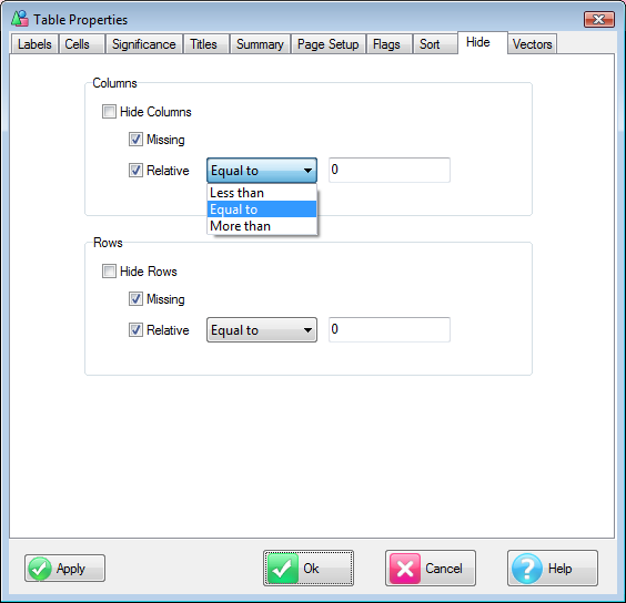
The Hide switches match the Hide Columns and Hide Rows buttons in the Display Status group on the Home tab of the Ribbon:
.When deciding what rows/columns to hide there are two conditions that can be applied.
Missing: the data is not defined and appears as an asterisk (*) on the table display.
Relative: hide conditionally, for example if 'equal to zero' or 'less than 3'.
If all data in a vector is missing or meets the conditional test (or both) then the vector qualifies for hiding.
Vectors tab
Vector settings are common to both tables and charts and they allow change to details on individual vectors.
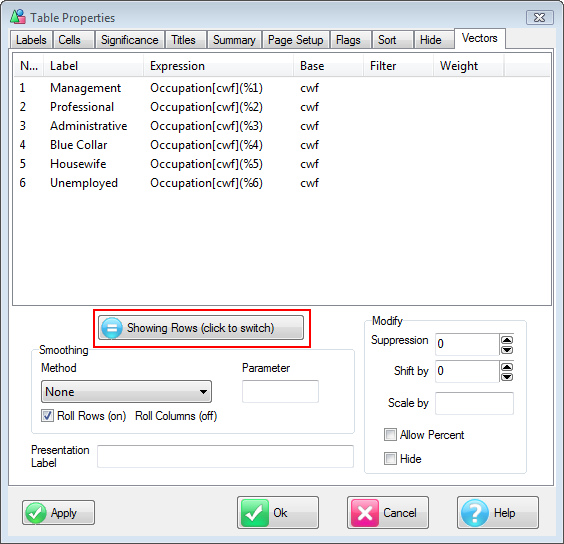
Showing Rows/Columns switches the vector set.
Click on one line to show or edit its details.
Multi-select is by the [Ctrl] or [Shift] keys.
Smoothing
Ruby currently supports two smoothing algorithms - Moving Average and Fixed Width Moving Average. They are both post averages meaning that a 4 point moving average returns the average of the current and the three previous points. Moving Average means keep going back until four non-missing points are in hand. Fixed Width means to use exactly the four previous points even if some are missing. Fixed Width is best for seasonal data.
Parameter: the number of points to roll.
Roll Rows (on) Roll Columns (off): Rolling can apply in only one direction. This switch determines if you are rolling rows or columns. This is actually the same switch as the chart XView switch on the Chart Properties | Series tab. It effectively means you are treating either the rows or columns as the series on a chart.
Modify
Suppression: You can suppress the display of the first n points. A common use of this is to hide the roll-in as n-1 points.
Shift by: You can shift all points forwards or backwards. This is useful for doing seasonal comparison, and for simulating a centroid or backwards roll - for a centroid roll left shift by half the moving average parameter, e.g. if the roll is 6, then left shift by 3.
Scale by: You can scale all points by any amount - useful for bringing very large or small numbers into a more convenient range.
Allow Percent: Show percentaged figures for this row/column when the appropriate ribbon Display Status toggles are set.
Hide: Hide/Show this row/column. This is the same as the Labels context menu Hide item.
Presentation Label
This is the customized label that will appear for the selected vector in Presentation mode. You can also change this with a Label menu item on context menu on the table, chart and specification form.
Chart Properties
The Chart Properties form is divided into a number of tabs.
Several these tabs have a thumbnail of the chart in the top left showing only those details relevant to the current tab.
All size and position values are shown as pixels, and are scaled to the chart's current window size.
If you change the window size the values will change accordingly.
All such measurements are actually stored internally, and in files relative to a theoretical window 100,000 pixels square, scaled down to the window, printer or thumbnail in which the chart is drawn.
Using pixels (rather than percents) allows absolute fineness for positioning.
Chart tab
The chart tab shows the largest pieces of the chart - the legends, graph box and background.
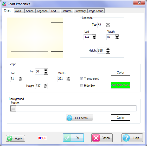
Legends: Position and size of the legend box.
Graph: Position and size of the Graph box.
Graph Colour: A separate colour to the background that will show if the Transparent flag is OFF, with no outline if Hide Box is ON.
Axis Selections: The colour of the patches you can drag out on any of the axes, and the colour used to indicate the results of the Show Me item on the Legend context menu.
Background: Select a graphic in any of the supported formats as a background.
If you browse for a picture using the … button, the selected picture will be copied into the job's Media directory if it is not already there.
Colour: Specifies a block colour.
Fill Effects: can be used to apply gradient shading.
Axes tab
The Axes tab shows details for one of the four axes, X1, X2 and Y1, Y2, shown with a highlight box around it.
Click on a thumbnail axis to change to it.
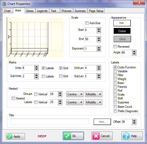
Scale
Axes may be showing the top or side labels from the underlying table (a category axis) or they may show a scale for the values from the body of the table (a value axis).
For a category axis, Start and End show the index of the labels in the underlying codeframe (first index is zero).
AutoSize will set these to zero and last label index.
For a value axis, Start and End are just numbers and AutoSize will look at all the series data to determine the largest and smallest values.
After AutoSize has determined Start and End points it organises the density of labels so that there are not too many and not too few.
Exponent is a power of ten for scaling the display.
If you have tiny numbers to show you can set it to -3 to show three decimal places.
If you have big values you might set this to 3 to show thousands.
When you change the Exponent value you will see the Start/End/Units/Subunits changing to match.
This is because the scale is always whole numbers.
So if you want to show 1 decimal place in a range of 2 to 5 the scale will change to 20 to 50 so there are enough 'ticks' to represent 2.0 to 5.0.
Appearance
Each axis can have a different colour, font and grid colour. The labels can be at any angle.
Reversed: Normal axis directions are left to right, bottom to top. You can reverse the display (without changing the underlying table) with this switch.
Marks
You can set how often you want Unit and Subunit marks and whether each of these has labels attached or grid lines attached.
UnitLen and SubLen control the length of the tick marks.
Nested
For category axes you can switch to Nested display and the axis labels will look the same as they do back on the underlying table.
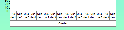
The settings here then allow fine adjustment of the space used by the groups and labels and the alignment of the text.
Labels
The axis labels are usually just the code label but it can often be convenient to build a label from any information about the underlying table vector, such as the same series differently filtered.
Title
You can supply a title for your axis that will be vertical text beside vertical axes and horizontal text above or below horizontal axes.
The Offset is how far away this title is from the axis.
Series tab
The series tab is for changing the general type of the chart and all cosmetic features for the series.
Click on a series legend in the list on the left to show its details.
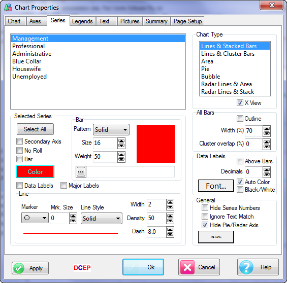
Many different chart types can be created using combinations of these settings.
Chart Type
XView switches between which of the axes is category and value.
When ON, the X1 axis shows the column labels from the underlying table and the Y axes show scales for values within the table.
When OFF, the Y1 axis shows the row labels from the underlying table and the X axes show scales for values within the table.
XView set to ON shows vertical bars and horizontal line series, and OFF shows horizontal bars and vertical line series. You may need to invert the top and side specifications to get the required layout. The easiest way to convert column bars to horizontal is the Flip item on a chart's context menu.
You can select from a variety of chart styles and set some overall values.
All Bars
Bars can take from 1 to 100% of the space available so you can have them thin or fat.
Bar Outline draws a one-pixel black line around any of the bar, area or stack styles.
For Cluster bars you can set the amount of overlap.
Data Labels
You can set the font and decimals for data labels. The colour can be a single colour stored in the font or two styles of auto-colouring.
Above Bars: show data labels above bars instead of inside
Decimals: decimals places for label values
Font: font to use for data labels (including colour unless auto)
Auto Color: for bars, labels are a contrasting colour; for series or above bars labels are same colour
Black/White: if Auto Color is ON just make labels black or white for best contrast
Data Labels / Major Labels
On the right you can turn Data Labels on/off for each series.
Major Labels means the values will only be shown on major axis ticks - handy for a dense category axis.
Significance always shows on every point and only when significance is turned ON.
General
Hide Series Numbers to show just the legend.
The Ignore Text Match switch turns off text matching for this chart.
Text matches are specified on the Job Series tab of the Preferences form.
Radar and Pie charts can hide or show the category axis. Hide for a cleaner display. Show to drag the ends as a way to limit the number of plot points.
Multi-Pie charts have a label next to each pie. The label font is set here.
Series
Any changes apply to all selected series.
The All button is a quick way to select all series so you can switch them all to bars, or all to a secondary axis, etc.
Secondary Axis means this series will be plotted against Y2 rather than Y1 (or X2 rather than X1 if XView is OFF).
No Roll protects this series against chart-wide roll settings (useful for inserted constants such as GRPs).
Bar switches between bar and line mode for the Lines & Bars styles.
You can set the series' colour, line width, line style, marker, marker size, bar pattern and pattern size. Note the blank marker at the top of the drop down for No Marker.
Bar
You can select from a variety of bar fills or an image (by selecting the last “Image” pattern) and adjust the size and weight of the tiling.
The Size setting is window-relative. If you change the size of your chart window the bar pattern or tile will change to follow the scale. This is so that printouts will be as close to WYSIWYG as possible.
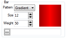
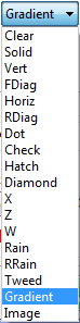
Line
You can select from a variety of markers (or none - the first item) and set the size.
You can also select a variety of line styles.
Width: the line width in pixels
Density: the relative space in dash and dot styles
Dash: the relative length of a dash in DashDot styles.
Set Style to Dot and Density to 1 for a scatter plot.
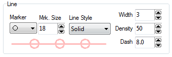

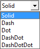
Legends tab
The Legends tab is for changing how legend text is generated and displayed.
You can change the style and appearance of the legends, but not the position. To change position, use the Chart tab or a mouse drag.
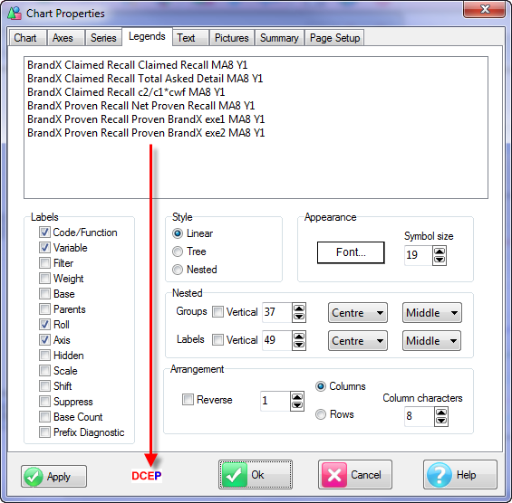
Use the DCEP button to cycle between the Diagnostic, Code-Expanded, Expanded and Presentation versions of the labels.
Note that this is only a local DCEP button and is not connected with the Display Status Label Mode setting on the ribbon.
Labels
The legends will be generated from whatever elements you have checked. If nothing is checked, just Code is used. This is most likely to be suitable, as usually the code label is all that is needed.
For comparison charts, which often have the same code label from several different variables, selecting Variable will help to distinguish them.
Filter, Weight and Base are details from the specification - you might have the same series filtered a few different ways.
Selecting Parents shows parent levels of hierarchic variables.
Selecting Axis shows which axis the series is plotted against
Roll, Hidden, Scale, Shift and Suppress will add those qualifiers to the legend if their values are non-default (zero or one depending on the item).
Style
Normal legends are Linear (and can be reversed with the Reverse switch) but you can have them Nested and they will appear just as they do on the underlying table.
Tree Style shows a copy of the top or side specification tree in a normal Tree View.
Appearance
One font is used for all legend text, set here. Symbol size is the width of the line or bar marker against each legend in pixels.
Nested
The Nested settings organise how the space is used for Groups and Labels and specify the text alignments.
Arrangement
Legends can be Reversed without changing the underlying table.
Normally, legends are in one column but you can organize for multi-column or row legends by changing the number and settings.
For multi-column legends the row height is determined by the height of the legend box.
For multi-row legends the column width is determined by the Column characters setting.
Text tab
Text added to a chart from the right mouse menu can be edited for properties other than the text itself here.
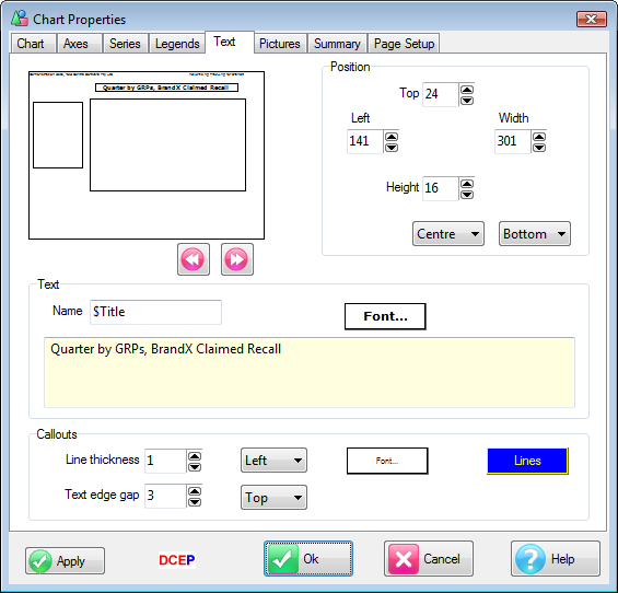
Each text item appears on a chart in a borderless box.
The text wraps around inside the box, avoiding splitting words if possible.
The current text item is shown with a selected box around it on the thumbnail.
Click on another text item to select it or use the << >> controls to cycle through all bits of text (useful if you have accidentally shifted one off screen).
Position
Changing the size of the box will change how the text wraps.
This can sometimes differ on different size windows, because of a font jumping a size as some threshold is passed, but the control is usually very good.
You can also change how the text is oriented within the box using the alignment controls.
Text
Each text item has a name. Names beginning with a $ are automatically generated.
If this is the case, the larger field will have a yellow background which indicates that you cannot edit the text.
$Name: the filename of the chart
$Title: the list of variables in top/side
$Filter: the overall filter
$Weight: the overall weight
$Roll: the common roll applied to all series
$Job: the job name
$Date: the date
$Time: the time
$DateTime: both date and time
$Base: the headcount (filtered but unweighted) of cases
The text generated for many of these also depends on the Label Mode setting.
Callouts
Callouts (often called events for date variables) are special text boxes with a line joining them to the category axis.
They belong to a code from the variable (or a date for a period variable).
You can change font, line colour and thickness and how the text is oriented within the box.
Pictures tab
Graphics added to a chart from the right mouse menu can be edited for properties other than the text itself here.
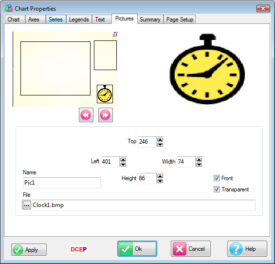
Each picture appears on the chart in a box. The selected picture is shown with its box drawn. Click off the picture to remove the selected box.
Click on another to select it or use the << >> controls to cycle through all pictures (useful if you accidentally shifted one off screen).
If the width or height of the picture is negative it will be flipped horizontally or vertically.
Pictures can be at the front or the back, which means that they are drawn before or after everything else.
Most pictures can be transparent but some types cannot. Different file formats indicate the transparent colour in different ways.
Some file types, such as bitmaps (*.BMP), use the bottom left pixel as the transparent colour.
Icon files (*.ico) cannot be resized. All other types can be resized by dragging the selection box edges.
Every picture has an internal name which can be used in scripts to identify it programatically.
Summary tab
Every chart can have a summary table either attached to an axis or as a floating window.
Specifying the calculations for the rows and columns is done in the Summary Planner.
The summary table's cosmetic settings are shown here.
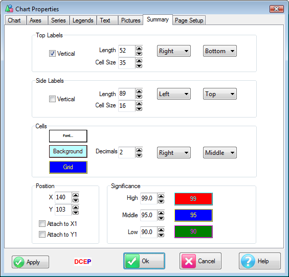
Top/Side Labels
The text in the labels can be vertical.
Length is the height of top labels or the width of side labels.
Cell size is width for top labels and height for side labels.
Text layout is set using the alignment controls.
Cells
Only one font is used for the entire table, specified here.
You can change the Background and Grid colours, also set the number of decimal places to use and the alignment of text in the cells.
Position
The XY position of the top left corner can be set or you can attach the summary table to either the X1 or Y1 axis where it replaces the axis labels.
This can be extremely effective in showing two sets of related information in a very coordinated fashion.
For instance, you might have a chart of weekly figures and attach a quarterly summary table to the X1 axis.
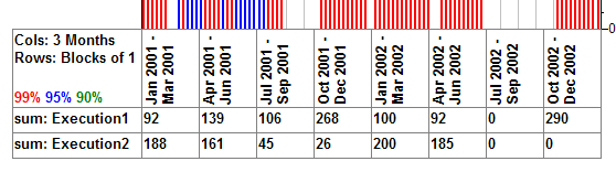
Significance
You can set the significance levels and colours to anything here. Any cell that is significantly different in the table will be colour-coded to indicate this.
Page Setup tab
These are the print settings that will be applied to hard copy if Override Batch Print Settings is ON.
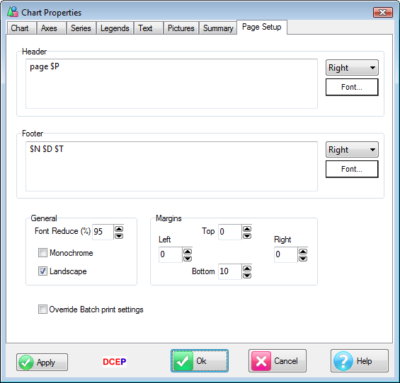
Header/Footer
This is the text that will appear as a header or footer on the printed page.
You can force white space by entering extra Returns and you can insert some dynamic information with substitution text.
$D is the date
$T the time
$P the page number (for batch printing)
$N is the file name.
You can set alignment and font for these as well.
Margins
Printers vary somewhat. If more spare selvedge space is needed, that can be set here.
Fonts
Printers also vary in how they treat fonts.
Often fonts seem bigger on paper than on screen so you can make an adjustment here to reduce the size of all fonts.
Monochrome: This forces all fonts, lines and patterns to black, and the background and graph box to white.
Pictures are left alone because most printers handle grey scaling automatically.
Landscape: Usually charts are printed one to a page in landscape mode.
When printing batches of charts, if two charts in a row are set to Portrait (Landscape off) they will both be printed on the one page at half size.
Override batch print settings: When batch-printing Ruby usually uses the settings from the Preferences Job Batch Print form for the entire run.
If you have a chart with particular print requirements you can set this switch ON.
Perceptual Map Properties
Access the Perceptual Map properties from the right-mouse context menu, pressing F3, or by clicking the Report Properties button on the toolbar.
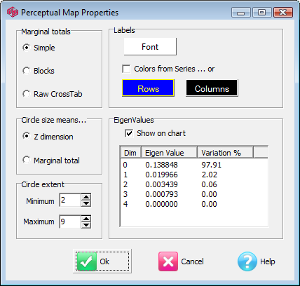
Marginal Totals
Correspondence Analysis usually gives a good indication of the relationship between row and column categories.
The analysis begins by calculating expected values and chi square contributions. This can be done as a simple table or by using Ruby table information.
Simple means that the table is treated as a stand-alone entity and the expected values are determined from row and column totals of the visible cell values only - what you see is what gets used.
Blocks means that if the table has multiple variables on an axis, then the totals are calculated within each variable block. This avoids double counting. Again, what you see is what gets used.
Raw CrossTab means that the expected values are determined using the totals from the underlying Ruby raw crosstabs.
If you have omitted some codes in the specification, their counts (and Not Established too) are nonetheless included in the row and column totals. In this case, what you see is not all of what gets used.
For example, if a variable has a code frame of 100 brands, but you are interested in only a few, you need to decide if the totals for calculating the expected values are to be taken from the raw crosstab totals of all 100 brands, or from just the few which you have selected.
For a table with multiple variables on an axis you should select either Blocks or Raw CrossTab.
Selecting Simple for a table with a demographics banner would in general be wrong, because the same respondents could be in more than one column.
There is nothing to prevent this, however, since for other multi-response variables (such as for a map of brand share), it may be reasonable and appropriate.
Circle size means...
Z dimension: large circles are above the plane and close to you, small circles are far away
Marginal Total: the circle size effectively shows the base size
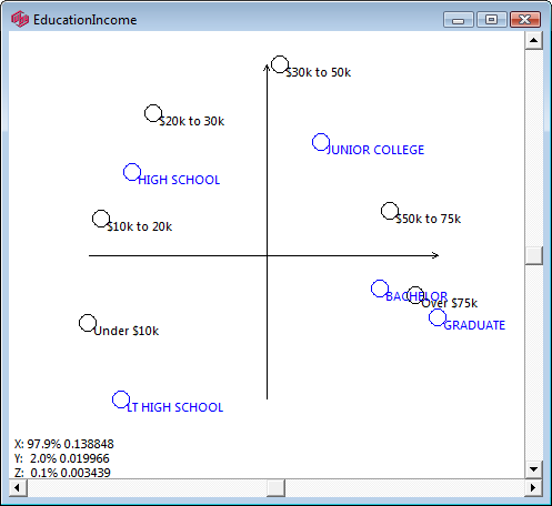
The same chart above with circle size = total shows the sample is evenly distributed.
Circle Extent: the maximum and minimum size for a circle (in pixels at the current window scale)
Labels: the font and colours for labels.
The map above has one colour for the rows and another for the columns.
If Colors from Series switch is on, the points take the colours of the underlying chart series.
On the chart Properties|Series tab you can change the colour of any series.
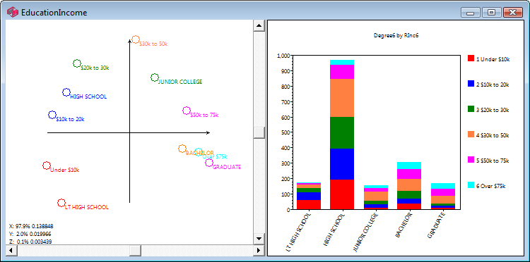
These are either the row or columns of the table depending on the X View switch.
This determines which axis is the Independent one.
With X View ON you get vertical bars, with it OFF you get horizontal bars.
NB: This is not the same as Flip - that does change the X View switch but also swaps the variables between top and side.
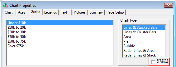
Right click on the chart and select Properties - don't use the toolbar properties button because that opens properties for the first view which in this case is the map
On the Series tab change colours for the current series
Change the setting of the X View switch
Click OK to close the form and effect the change of view
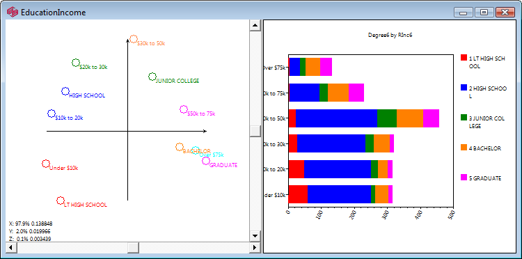
Common
Common properties apply to both tables and charts. Since all common properties are also table properties, the Common Properties form is the Table Properties form with non-common tabs removed.
See Table Properties.
Callouts
With a chart in focus, click the Callouts button
on the Properties group of the Home tab to open the Chart Callouts form.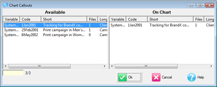
On the left is the list of callouts available for the independent variable (X axis if XView switch is ON, Y axis if not).
If this is a date variable the list will also include all callouts in the SystemDates variable.
On the right is the list of callouts on the chart.
Drag from left to right to add some more, or press [Delete] on the right to remove some.
See Edit Callouts.
Gauge Properties
The properties form for gauges lets you control some parameters and cosmetics.
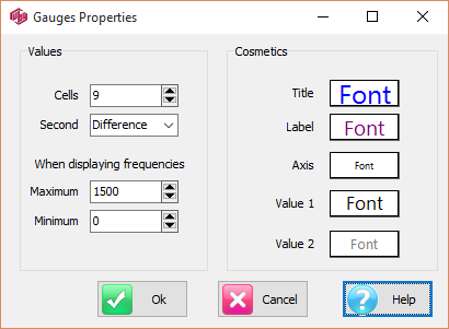
Cells: show at most this many cells (one per row from the table)
Second: show the second column as a difference or report it directly
Maximum/Minimum: the scale for the gauge when showing percents is always 0 -100, but when showing frequencies you need to set the scale using these controls
Fonts: controls text fonts
Display Status Group


 : Toggle on or off the display of the: Table Chart Map Gauges


 : Toggle on or off the display of: Frequencies Column Percents Row Percents Significance : Toggle on or off Sort Rows Sort Columns . Right-click to reverse the sort order. : Toggle on or off Hide Columns Hide Rows
 For

see Label Modes, Summary Planner, Global Filter.
Label Modes
Labels on reports can be in one of four modes, selectable from the Display Status Group on the Home tab of the Ribbon:
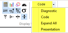
The default Label Mode is a global setting, stored in the Windows registry and set on the System General tab of the Preferences form (under the Ruby Application Menu):
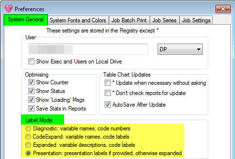
The appearance of the labels in each of the display modes of the tables below is illustrated in the following sequence.
The top variable has:
file name ABA
description Aided Brand Awareness
local Presentation text Recognition when shown brands
The first code has:
code number 1
code label BrandX
local Presentation text Home brand
The last column is a function:
expression sum#ABA(2/3)
local presentation text The competition
The side variable has:
file name Gender and AKA GEN
no description or presentation text
Diagnostic mode:
Variables appear as AKA or file name, codes as numeric. This is useful for DP analysis where the label meanings are less important than the structure of the data.
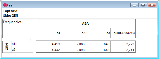
Code-expand mode:
Variables appear as AKA or file name, codes as labels. This is a comfortable interactive working mode for researchers where variable descriptions might be too bulky to read easily.
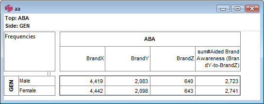
Expanded mode:
Variables appear as descriptions, codes as labels. This is useful for jobs where the variable names are arbitrary and not self-documenting, such as X23, or SQ32a.
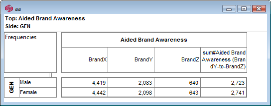
Presentation mode:
Any presentation text set globally or locally is used. This is usually where the researcher has used text more suitable to presentation or client delivery. If no presentation text has been entered, the display in Presentation mode will be the same as that seen in Expanded mode.
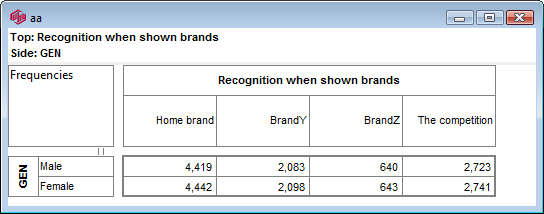
Summary Planner
A smaller summary table can be attached to any table or chart. Each column is made from one or more columns of the original table and each row from one or more original rows.
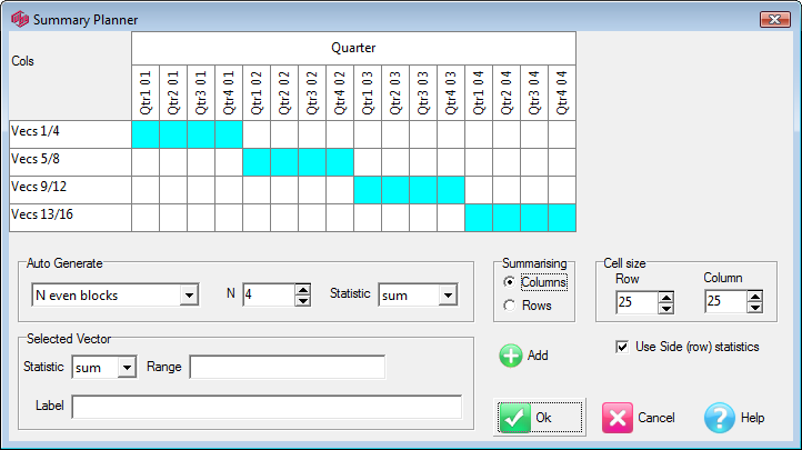
The Summary Planner specifies which rows and columns are summarised and what calculations are used.
These pictures show a chart of Quarter by Region being summarised into four even columns and one row per original row.
This is the default summary.
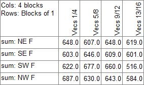
The column and row summarising is done independently, according to the on/off status of the Summarising radio buttons.
The blue squares show which of the original rows or columns (along the top) are incorporated in the summary rows or columns (down the side).
In the above, the first summary column (labelled Vecs 1/4) is composed of the first four columns from the table (labelled Quarter1 to 4).
And below, the first summary row (labelled sum: NE F) is composed of just one row of the original table (labelled NE).
It can be a little confusing at first getting used to sometimes seeing rows across the top and columns down the side.
The top of this display is always from the originating table (rows or columns) so the labels will usually be nested.
The side of this display is always from the summary table (rows or columns) and hence the labels will never be nested.
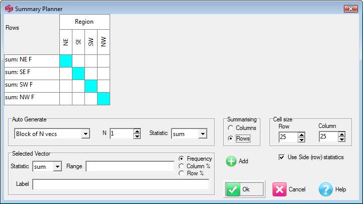
Usually the sets of rows and columns are auto-generated but you can also make manual selections.
Use either the controls in Auto Generate or those in Selected Vec, not both, although you may start with an Auto Generate selection and then make manual changes in Selected Vec.
You may also generate the columns but manually select the rows - they are quite independent.
Generated summaries incorporate additional rows or columns that might result from updates to codeframes and are simple to set up.
Manual summaries allow specification of every detail and can accommodate exotic requirements.
To auto-generate, select one of the summarising plans and a statistic to use in combining cells.
This is commonly Sum but the standard set is available for imaginative uses.
(A vector is a row or column.)
N even blocks: The available number of vectors is divided into N blocks, as evenly as possible.
The example has 16 columns in four even blocks resulting in 4 columns per block.
In the example above, N=3 would create three blocks, the first two comprising 6 columns and the last having 4 (making 16 all together).
Block of N vecs: Each summary block contains N vectors.
In the example above, N=2 would create eight summary columns each comprising 2 original columns.
Block of N Days, Weeks, Months, Years: These are specially made for Date (MJD) variables.
For example, if the X axis is a date variable you can summarise it by calendar periods.
Weeks do not go evenly into months, but as long as the right variables are available all the work is done for you.
You can think of date variables as two types: day based (Days, Weeks) and month based (Months, Quarters, Years).
If your original plot is day based and you want a month based summary Ruby will run an additional table in the background. e.g. all your side variables against the Month variable.
The name Month is not mandatory - Ruby just looks for a variable with a date cycle of one month.
Selections: Each summary block is one of the selected patches on the corresponding axis on the chart.
This is just the selections, not the gaps in between.
Selections and Gaps: Each block is a selection or a gap from the chart.
Selected vs Unselected: This results in just two blocks.
The first is comprised of every selected point on the chart and the second is every unselected point.
The switch Use Side (row) Statistics determines which statistic selection is used to combine cells.
e.g. You might have a summary cell whose row is made from three original rows and whose column is made from two original columns.
Thus there are six cells from the original table to be combined in some way to make the single summary cell.
The row may have the Sum stat and the column may have Avg.
If the switch is ON you get the Sum of the six cells; if it is OFF, then you get the Average.
The labels of the summary table indicate what statistics have been applied.
You can tell that Row Stats is on in the table at the beginning of this section because all the row labels begin with “sum”.
Whatever rows the originating table or chart is showing get reproduced in the summary.
A table showing Frequencies and Column Percents will deliver two summary rows for each block.
The first will have an 'F' suffix ad the second a 'C' suffix indicating Frequency and Column Percents.
The generated labels depend on the plan and the number.
For date summaries the labels are the start and end dates of the period.
For even-blocks and blocks-of, if there is only one vector in the block the label is the label from the vector (for example NE in the rows example above), if more than one then it is like 'vec 1/4' indicating the range of rows or columns.
The selection types get a range expression like 'vec 2/5' except for Selected-vs-Unselected, which has just those words.
If the RowStats switch indicates that these statistics are being used, the name of the statistic will prefix the label.
For row summary blocks, the letters F, C and R are suffixed indicating that the summary is of the Frequency, Column Percent or Row Percent figures.
If you make any of the following manual changes, the drop down in the Auto Generate section will switch to '----------' meaning no generation.
You can manually set which original vectors contribute to each summary vector by clicking in the main table.
The blue patches toggle on/off to indicate inclusion and you are free to overlap or leave unused as you choose.
Alternatively, type the range as numbers in the Selected Vec section.
You can change labels and set different statistics and frequency/percent switches for each vector.
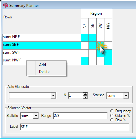
There is one quirk resulting from this flexibility: the blue squares can appear to be stubborn and refuse to change.
If the cursor is in the Range or Label fields and you attempt to click a blue/white square in the selected vector (for example if you click anything in the South row above) nothing changes.
This is because the click in the grid causes an Exit message from the Range or Label, which refreshes the display to match those fields, thereby preventing any change.
To defeat this, select a different vector first (by clicking on the label) or get your cursor out of the Selected Vec section (for example in the N thumbwheel or the Cell Size section).
Add summary vectors from the context menu by clicking the Add button.
Delete summary vectors by clicking the right-mouse on the vector and selecting Delete.
Resize the display using the same mouse functions as on all other Ruby tables.
You can drag-resize the top or side labels, the width of the first column or the height of the first row, and the bottom and right edges.
Alternatively you can change the numbers in the Cell Size section - very handy if accidentally dragged to be too small.
For a click-by-click example of using a summary table to determine if an advertising flight has made a significant difference, see the section Is it Significant? in the document Typical Ruby Analysis Session.pdf.
Global Filter
Enable or disable the current global filter as specified on the Preferences form. See Job Settings.
Font Group
The Font group on the Home tab of the Ribbon has settings for fonts for the active report. Some options change depending on the report type (table, chart, perceptual map or gauge). Font settings are also available on the Properties forms.
All Regions

Select from the dropdown list to adjust font settings for all regions or a specific element on the active report:
Font

Select a font from the list.
Style

Select a font style (Normal, Bold, Italic or Bold Italic) from the dropdown list:
Horizontal Alignment


Select left, centre or right horizontal alignment.
Vertical Alignment


Select top, middle or bottom vertical alignment.
Color

Select a font colour from the Color form.
Font Size


Increase or decrease font size.
Layout Group
Use these buttons to control overall / report-wide adjustment of:

 decimals up and down
 gridlines up and down (for charts the box area and for tables the grid)
 grid colour or chart plot area border colour
 table labels background colour
View Tab
The controls on the View Tab relate to window display and the look-and-feel of the interface.
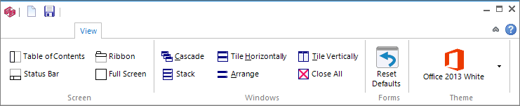
Screen Group:
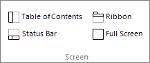
Windows Group:
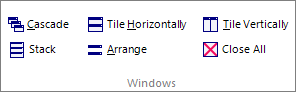
Forms Group:

Theme Group:
Screen Group
Table of Contents

Toggles the display of the Table of Contents (TOC) on/off
Ribbon

Toggles the display of the Ribbon on/off
Status Bar

Toggles the display of the Status Bar on/off
Full Screen

Displays the active report in full screen mode - the Esc key restores the normal report view
Windows Group
Cascade

Arranges the open reports cascaded in the report display pane.
Tile Horizontally

Arranges the open reports tiled horizontally in the report display pane.
Tile Vertically

Arranges the open reports tiled vertically in the report display pane.
Stack

Arranges the open reports one below the other in the report display pane.
Arrange

Arranges the open reports one below the other in the report display pane.
Close All

Closes all the open reports in the report display pane but leaves the reports in memory. See In Memory Form.
Forms Group
Reset Defaults
The major forms (Specification, Variable, Construct, Vartree) retain their last used position and layout.
This button is used to restore these major forms to their default positions.
Sometimes, if the last session was on dual monitors, but the current session is on a single monitor, forms on the second monitor at Ruby Close time will now be off-screen. Reset Defaults will bring them back to within the single monitor's view.
Theme Group
Themes Dropdown List
Select a theme from the dropdown list:
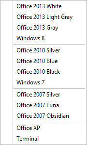
Tools Tab
The Tools Tab is for batch operations and other routine tasks.
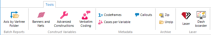
Batch Reports Group:

Construct Variables Group:
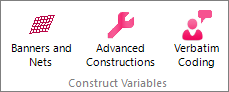
Metadata Group:
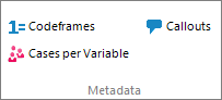
Archive Group:

Laser Goup:
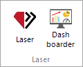
Batch Reports Group
Axis by Vartree Folder

Opens the Axis by Folder form.
Use this form to run custom banners by large numbers of variables. Use GenTab syntax (see the RubyAPI Help) to specify the top axis and the vectors for each variable on the side axis.
The fields here are saved with the job so they can be rerun at any time.
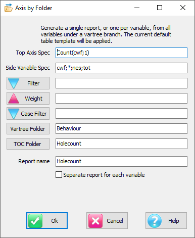
Top Axis Spec: The top axis for all tables.
Side Variable Spec: Each variable is run with this as its code range - e.g. Gender(cwf;*;nes;tot) then Region(cwf;*;nes;tot) etc
Filter: A table filter
Weight: A table weight
Case Filter: Optional case filter to apply to all generated reports
Vartree Folder: Select a branch of the Variable tree to list - empty means all
TOC Folder: Destination folder for the generated tables
Report name: Name of report if the Separate switch is OFF
Separate report for each variable: Check this to generate one table for each variable, otherwise it is a single table called Holecount with all variables down the side
Prefix: The separate tables are named by adding this prefix to the variable's name
Level: For a Levels job, the Levels drop-down list will be visible
Construct Variables Group
Banners and Nets

Opens the Banners and Nets form.
Advanced Constructions

The Advanced Constructions command exposes the full DP Construct Variables form to analysts.
See Construct Variables Form.
Verbatim Coding

Opens the Verbatim Coding form where automated verbatim coding is specified and run.
Banners & Nets Form
Banners and nets that are likely to be used a lot can be incorporated into new variables as a permanent part of the job. You could ask DP to make the new variables for you - or use the Banners and Nets form, which is a simplified construction device specifically designed to make it easy to net codes or variables, especially codes within hierarchies.
One thing that cannot be done on the Specification form is netting codes in a hierarchic variable. You can however do that in the Banners and Nets form.
Each time you create a new variable it is added to the bottom of the variable tree. DP users have rights to edit the variable tree - the new variables can be placed in whatever folder structure you request.
All constructions, detailed here, can equally be made or edited in the full Construct Form (available both on the Construct Variables group of the Tools tab and on the Tasks group of the DP tab).
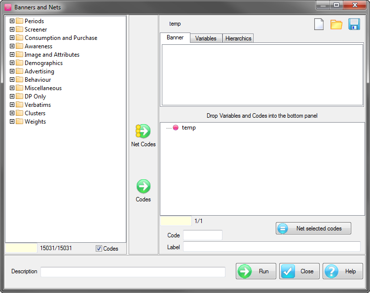
General
This form works in three modes (one tab for each):
Banner
Variables
Hierarchics
Banner mode: You drop variables or codes onto the bottom panel, gradually building a bigger and bigger codeframe. Each new code is given a new number (its original number if that hasn't been used), and you can change codes and labels and remove codes. You can net codes on the fly or anytime after. If you drop a code onto an existing one it is added to the net contributing to the existing code. When you click on a code in the bottom panel you see all the originating codes that will be netted in the top. You can remove some of these or drop more into the top. You can also highlight several bottom codes and click Net to merge them into one code (the last one clicked).
Variables mode: When you drop variables onto the top panel, their joint codeframe is displayed in the bottom panel (you can choose to allow all codes or just common codes). You can change code labels but not the codes, and you can delete codes but not add new ones. You can give your variable a name and description.
Hierarchics mode: You start by dropping a hierarchic variable into the bottom panel and then net codes within the hierarchic variable.
Loading and Saving
Saving is automatic when you click the Run button but you can Save
 explicitly any time you like.
 You can load a previously created variable to edit its definition simply by double-clicking it in the variable tree, or by clicking the Open button
near the Name field.If the chosen variable is a simple construction, the form is filled out and switched to the correct mode. If not, you will get a message indicating that Ruby cannot interpret this as a simple construction.
Banner: Netting Simple Codes
This is a quick way to build a banner variable, with or without netting any codes, as well as a way of netting codes to make a variable with a reduced scale.
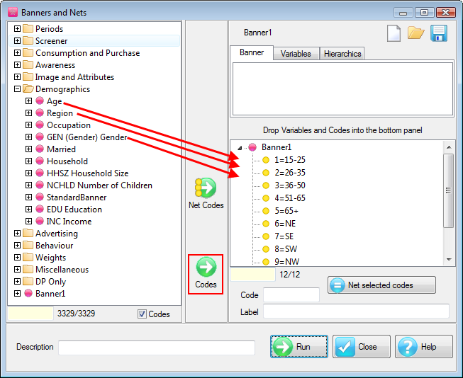
Make sure the Banner tab os selected
Open the Demographics folder
Drag Age, Region and Gender to the bottom panel (or select and click the Codes
 button)
NB: Each new code gets the next number available.
Click Run - save as Banner1 when prompted
The construction runs and the new variable added to the end of the Variable Tree.
When you click Run, if the variable name is temp you will be prompted for a save name.
If you want to run an existing net as another name you will need to first
Save it under another name. You get Overwrite? prompts anyway.Netting existing codes
This has made a useful banner variable straight away but you might want to net some of the Age codes to make fewer categories. To net the first three codes into a new one that you might label 'Young':
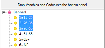
Highlight the first three codes using standard Windows [Ctrl] or [Shift] techniques
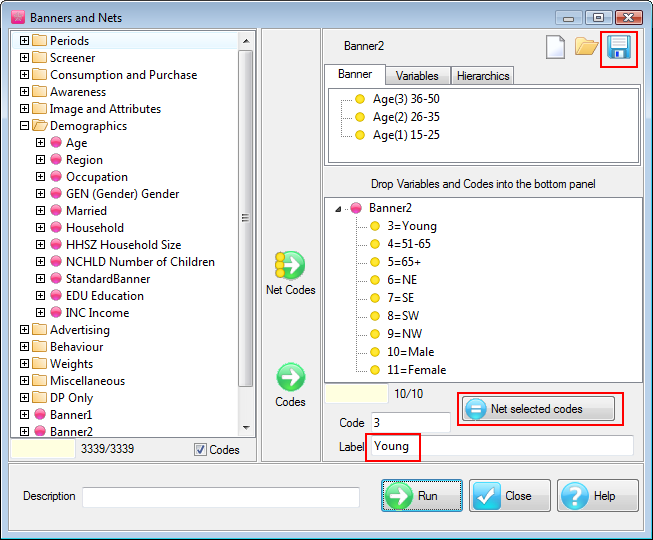
Click the Net selected codes button

This makes a new code that is the net of the other three (now in the top panel) keeping the code of the last one selected.
Change the Label to Young
Save
the variable as Banner 2 Click Run
The construction runs and the new variable is added to the end of the Variable Tree.
Netting as you drop
You can use the Net Codes
 button to net codes on the fly.
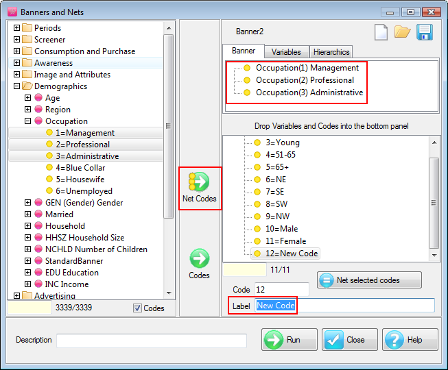
Multi-select some codes in the Variable Tree and click the Net Codes button. This makes a New Code again and shows the codes it came from in the top panel.
Editing Nets
Every code in the new variable is potentially a net and the top panel always shows the composition of the selected node.
All copied nodes will have only one entry here.
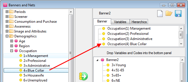
You can use this top panel to build up the netting by dropping other codes for the Variable Tree and you can [Delete] any codes here to change the netting.
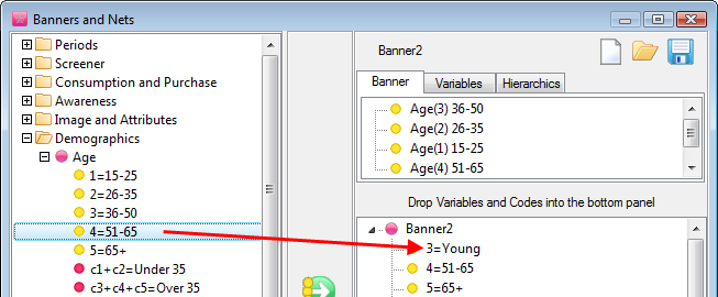
You can also build up nets by dropping codes from the Variable Tree directly on codes in the new variable.
You can change the Code or Label of the new codes at any time by clicking on the code and editing the fields.
Netting Variables
You may have several variables with the same codeframe and want to net them together into a new collective variable.
This exercise will net some advertising variables that record when particular details of an ad were mentioned.
The original variables are for each brand in turn.
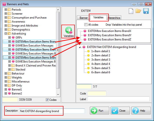
Make sure the tab at the top is set to Variables
NB: Changing the tab always starts a new variable as if you had clicked the New button
 .
.Open the Advertising folder
Drag EXITEMbrx, EXITEMbry and EXITEMbrz to the top panel or select them and click the Variables button

The first one dropped provides the initial codeframe. Subsequent ones may increase or reduce the codeframe depending on the All Codes switch.
If All Codes is ON then any codes in the dropped variable not in the current set are added. The codeframe increases when necessary to accommodate all codes.
If All Codes is OFF then any codes in the codeframe that are not present in the dropped variable are removed so that the set is only those codes common to all contributing variables.
When you click on a code its label is presented in the Label field for editing.
NB: This is a Hit-Enter-For-Next field so you can edit, press Enter and the next code is presented without having to click it.
When selected, pressing [Delete] removes the code (unless focus is in the Edit field).
Type Net EXITEM disregarding brand in the Description field
Save
the variable as EXITEM and Run - or Click Run and save as EXITEM when prompted.The construction is run and the new variable is added to the end of the Variable Tree.
Netting Hierarchic Codes
In Hierarchic mode you start with one hierarchic variable. You cannot add extra codes from other variables (that doesn't make sense because they are outside the hierarchy) but you can net codes within and remove, relabel, or recode as desired.
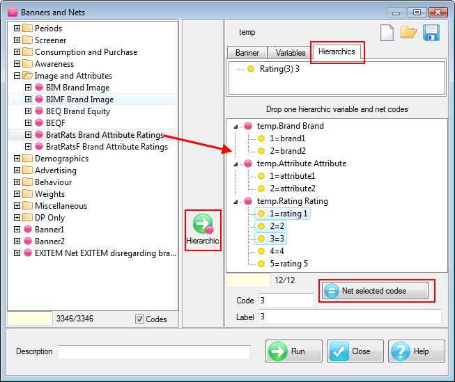
Make sure the tab at the top is set to Hierarchics
Open the Image and Attributes folder
Drag BratRats to the bottom panel or select it and click the Hierarchics button
Highlight the first three .Rating codes in preparation for netting them to a single Disapprove code
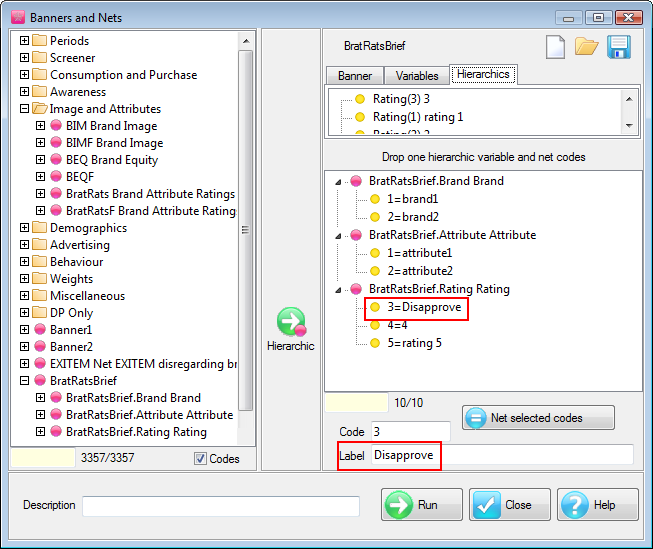
Click the Net selected codes button
Change the Label to Disapprove
Click Run, save as BratRatsBrief
The construction is run and the new variable added to the end of the Variable Tree.
Close the form
Advanced Constructions
See Construct Variables Form.
Verbatim Coding
Verbatim Coding is a tool for coding and editing verbatim variables within a Ruby job.
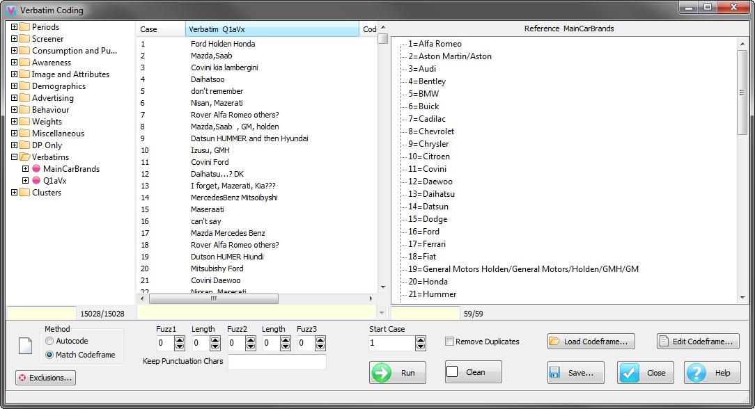
At import time, verbatim variables are pre-processed by sorting the response strings alphabetically from lowest to highest, and then allocating a code to each string in order.
For continuous tracking jobs, each wave is sorted independently (otherwise already allocated codes could change), and then coded from the next available code onwards. Such variables generally accumulate a large number of unique single responses. For example, the variable Q1aVx in the Ruby Demo job, for a Brand Awareness type question of car manufacturers is:
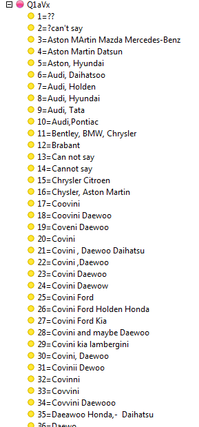
Verbatim Coding takes such a variable and recodes it either by each unique word, or by fuzzy string matching against a reference code frame.
NB: Recoding by each unique word operates on all cases, so it is not appropriate for tracking jobs, because a rerun after a case data update could change existing codes.
Autocoding decomposes each response string into its individual words, pools all the words, sorts alphabetically from lowest to highest, and then allocates codes from first to last, starting with code 1. The last code will thus also be the number of unique words found.
Exercise: A Coding Example
The variables in the Demo job for this walkthrough are in the folder Verbatims:
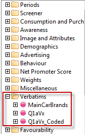
NB: If you are not the first to do this exercise on your installation of the Demo job, and have both the files RubyJobsDemoVerberator_Exclusions.txt and RubyJobsDemoVerberator_Exclusions.xxx, then delete the *.txt version.
If you have onlyRubyJobsDemoVerberator_Exclusions.txt, then rename it to RubyJobsDemoVerberator_Exclusions.xxx.
If you still do not have a RubyJobsDemoVerberator_Exclusions.xxx, then you will need to restore it from your original Ruby download.
Autocoding
To autocode Q1aVx
Drag and drop Q1AVx to the central Verbatim panel
Select the mode as AutoCode
Click Run
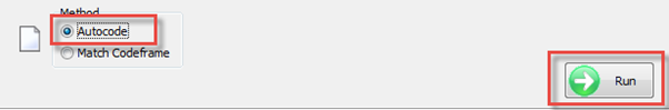
In a second or so the coded version and code frame are displayed. Case #1 responded 'Ford Holden Honda', which are codes 74, 91 and 95 respectively. Case #8 also has “holden”. Case#11 and #20 both also have Ford.
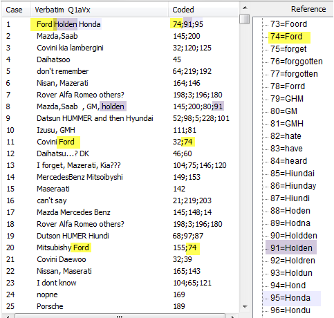
The item count at the bottom right indicates that 249 unique words were found.
Autocoding is an exact process. Words which are a letter or two different are taken to be different words. Thus, to a human Holden and Holdden are semantically the same, but autocoding has them as distinct items, coded as 90 and 91.
Save the Autocode
Click the Save button
The coded variable is saved as Q1aVx_Coded and appended to the vartree.
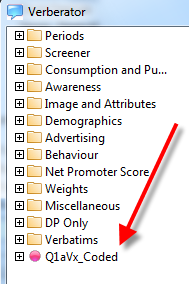
Q1aVx_Coded can now be used in Ruby.
A common first step is to net the various spellings of the various brands.
For Daewoo, the candidates for that as the intended brand in a respondent's mind would be:
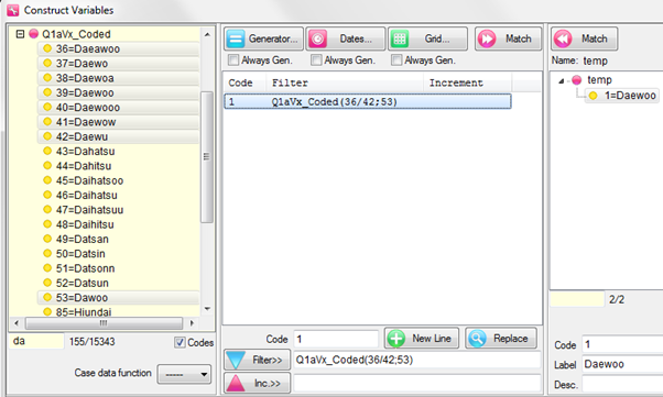
This is also a good way to do a thematic analysis - net all positive/favourable words, all negative/unfavourable, etc.
Another good preliminary move is to chart the sorted frequencies.
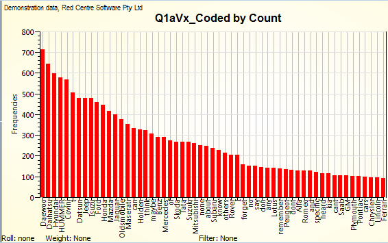
Load a Verbatim Variable
Double click Q1aVx or drag it to the Verbatim column
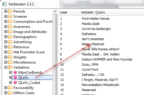
The variable is decoded back to its original source text, exactly as delivered by the respondent at each case, and loaded into the Verbatim column of the middle panel.
The decoding can be confirmed by looking at the case data for Q1aVx.
Right click on Q1aVx and select Data
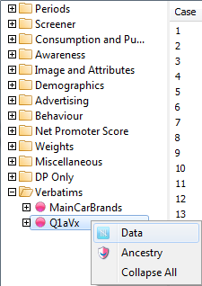
The dataform displays:
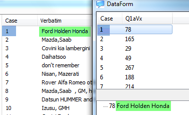
Autocoding is suitable for the analysis of well-formed texts, such as novels, focus group transcripts, etc, but it is not so good for mal-formed text such as is often found in respondent verbatims.
Unfortunately, there is no practical limit to the number of ways a respondent can mis-spell a word, or introduce a typo, and they cannot all be anticipated up front.
Match Code Frame
The second method, Match Code Frame, shows how to handle such variety by using fuzzy logic matching instead.
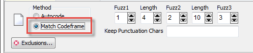
This matches the verbatim text against a predefined reference code frame.
The reference code frame contains all the intended targets for matching, and the Fuzziness parameters set how far away (measured as the number of letters which must be changed/inserted/dropped/swapped) the actual source text can be.
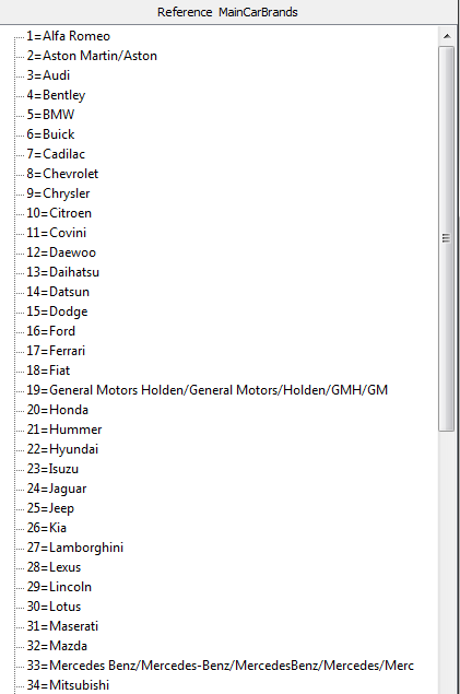
A fuzz setting of 0 means an exact match must be found.
A setting of 1 allows for one difference, a setting of 2 allows for two differences, etc, where a difference is at least one of change, insert, drop or swap.
A setting of 3 or more may start to introduce false matches, because with fuzz=3 'cat' will match on 'dog'.
In the example variable, GMH will match on BMW with fuzz=2 because GMH->BMH->BMW in two moves (G->B, H->W).
In general, the longer the string, the higher the fuzz factor can safely be.
To handle this, there are three fuzz factor settings, with length values to determine when they are applied.
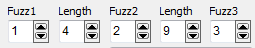
These settings mean that for character strings of 1 to 4 characters, one difference is allowed, for strings of up to 9 characters, two differences are allowed, and for 10 or more characters, three differences are allowed. The only relaxation so far on exactness is a case-insensitive compare.
The settings below look for an exact match against the master reference codeframe for all strings up to ten characters, and allows one difference for more than ten:
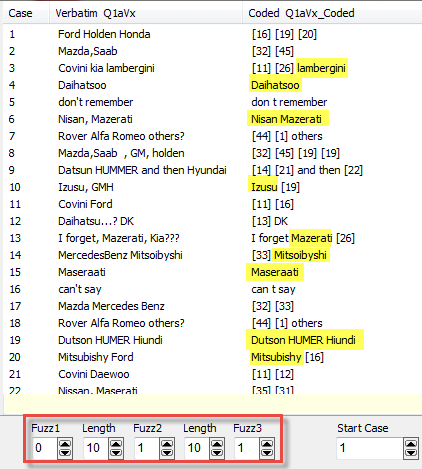
As you can see, every misspelt car brand in the verbatim response has not been coded, so these are not useful parameters for this set of verbatims.
These settings, on the other hand, do an excellent job on Q1aVx:
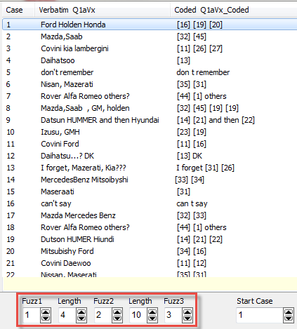
All human-identifiable text strings in the above (cases 1/22) have now been correctly coded.
To see the effect of varying the fuzz and length parameters more closely
Change Fuzz3 to 2 and Run
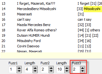
The string 'Mitsoibyshi' is 11 characters long, so two differences are allowed, but it takes three transforms to get from 'Mitsoibyshi' to 'Mitsubishi' (o->u, remove i, y->i).
At parameters 1, 4, 2, 10, 3, 'Izusu' at case #10, is correctly coded as 23. There are five characters, so up to 2 differences are allowed. The correct spelling is 'Isuzu' (s and z reversed, but they are not adjacent, so it takes two transforms).
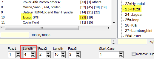
To see the effect of varying a length parameter
Change Length=4 to Length=5 and Run
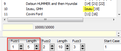
Strings up to five characters can now have only 1 difference, so 'Izusu', at five characters, and two differences from the master, is now not coded.
The most common values for the fuzz parameters are 0, 1, 2 or 1, 2, 3, that is, fuzz1Exclusion Lists
False matches on common words can be mostly prevented by creating a list of excluded words.
There can be many lists, stored as simple ASCII files.
Different variables in different jobs will need different exclusions.
A default file named Verberator_Exclusions.txt is checked for at run time, and if found in the job directory, then it is loaded automatically.
The phrases and words to be always excluded in this job are
have no idea
can't think of any others
cant think of any
cannot think of any
cant think of another brand
can't think of another brand
none specific
dnt knw
none
I don't know
I dont know
dont know
don't remember
dont remember
can't remember
cant remember
cannot recall
can't recall
cant recall
and
any
an
a
at
from
here
n/a
of
on
over
the
to
where
there
then
Apostrophes, as is so often the case, are something of a nuisance.
The default master list cannot go higher than the job level, because another job could have for example a brand item for a travel company named From Here to There.
To load the default exclusions file
Close the Verbatim Coding form
Copy RubyJobsDemoVerberator_Exclusions.xxx to Verberator_Exclusions.txt
Reopen the Verbatim Coding form
The name of the loaded Exclusions file is displayed.
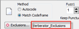
Looking at case #5 and case #9, previously there is some unwanted text.
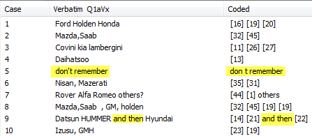
Running again, with the exclusions list loaded and with an apostrophe allowed, the redundant text is removed.
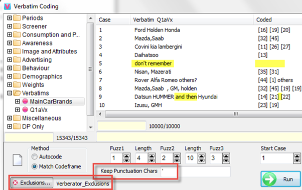
The text items don't remember, and and then are all cited in the exclusions file, so they no longer appear in the Coded column.
You can additionally load a variable-specific or job-specific file of exclusions to extend the defaults.
The name of the file is comma-appended to any prior loads.
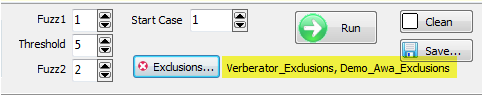
Add a Code Manually
The coded case data can be directly edited at any time by a double-click in the Coded column, or by dragging a code from the reference list on the right, and dropping it on the code string in the Coded column.
At case #139, there is an instance of Lamborghini as 'lambigini' which a human would identify immediately, but which would require reducing Length=10 to Length=8, so that, at 9 characters, the matching test would allow three transforms(i->o, insert r, insert h). But that could generate false positives, or miss more strings elsewhere than it is worth.
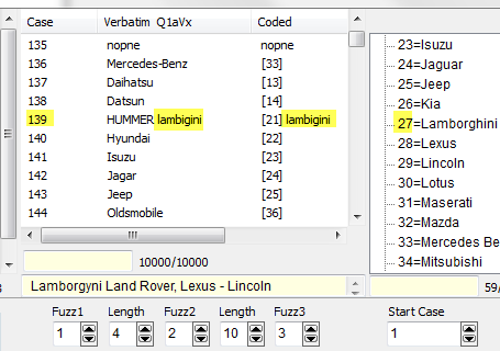
To manually override this
Drag code 27 to the centre panel and drop it on the Coded field for case #139
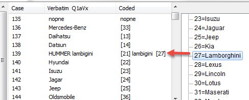
Edit the Codes
An entry against a case in the Coded column can be directly edited at any time.
To remove the text lambigini
Double click on the text in the Coded column for case #139
Remove the text
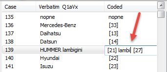
If there are many contiguous lines to edit, pressing Enter drops the edit field to the line below.
If manually entering a code, make sure to put it in square brackets, or else it will be cleaned as extraneous text.
Clean and Save
The brands indicated by the reference code frame are now comprehensively identified, but there is still quite a bit of extraneous text.
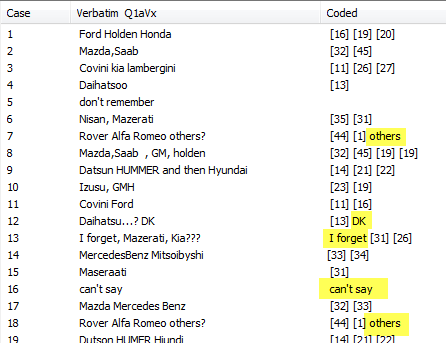
To get rid of the remaining text, and to convert the [16] [19] [20] etc to the final Ruby format of 16;19;20
Click the Clean button
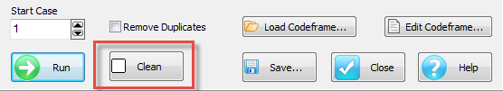
The Coded column redisplays as:
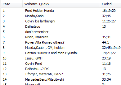
Note that you can only clean once. If you clean again, all the codes will be lost, and you will have to rerun to restore them.
Click Save
The coded data is saved to Q1Vx_Coded. You do not have a choice about the “_Coded” extension.
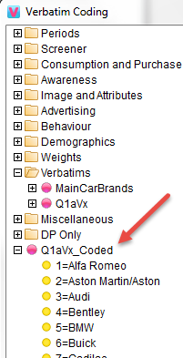
Remove Duplicate Codes
Depending on the nature of the variable, it may be appropriate to remove duplicate codes.
Check Remove Duplicates
Click Clean
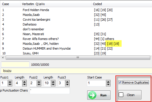
Case#8, previously displaying [19][19], becomes
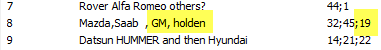
Check the Coding with a Table
A table of Coded by Raw, ie, here Q1aVx_Coded by Q1aVx, will quickly show how good the coding was.
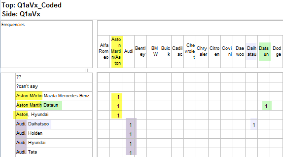
Load and Edit the Reference Codeframe
A code frame not already in the job can be loaded directly from the Load Codeframe button.
The current reference code frame can be edited for reorder, insert, delete, add new and change existing from the Edit Codeframe button.
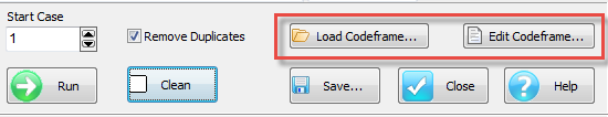
To help prevent false matches, the search order for synonyms should be from the longest to the shortest, as in:
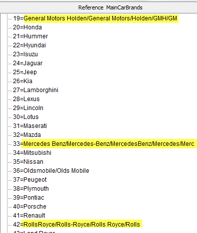
This ensures that substrings are found last.
Editing Human-coded Variables
A common scenario is that a human coder provides a file of coded verbatims which are then imported into Ruby, but on analysis refinements and possibly corrections are seen to be needed.
To handle this, Verbatim Coding allows any variable to be dropped into the Coded column.
This is a powerful but potentially dangerous facility - for example there is nothing to prevent dropping the codes from Gender against the verbatims from Q1aVx:
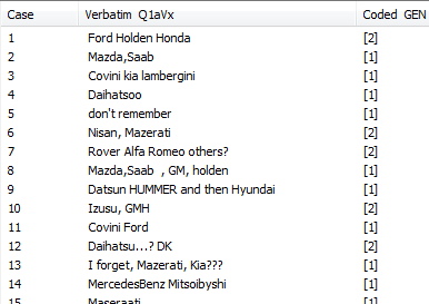
This produces nonsense, of course, but the Verbatim Coding procedure has no way of knowing what an externally coded variable has been named, so there is no way to protect against such a mis-assignment. It is assumed that you know what you are doing, and why.
To effect manual edits on a partially completed coding of a verbatim variable:
A - Drag the Reference variable (MainCarBrands) to the Reference panel
B - Drag the source verbatim (Q1aVx) to the Verbatim column of the middle panel
C - Drag the coded version of this variable (Q1aVx_Coded) to the Coded column of the middle panel
Make the required edits (you will need to highlight and delete [0] in each code since uncoded items are loaded with it by default.
Clean and Save
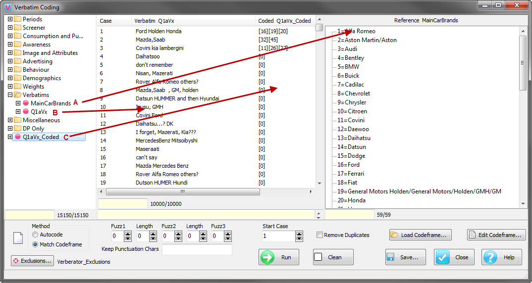
Updating Tracking Jobs
For tracking jobs, all code assignments from prior waves must be preserved.
To limit processing to just recent cases, set the Start Case value to the first sequential case for the update.
Double-click Q1aVx_Coded to reload with all parameters
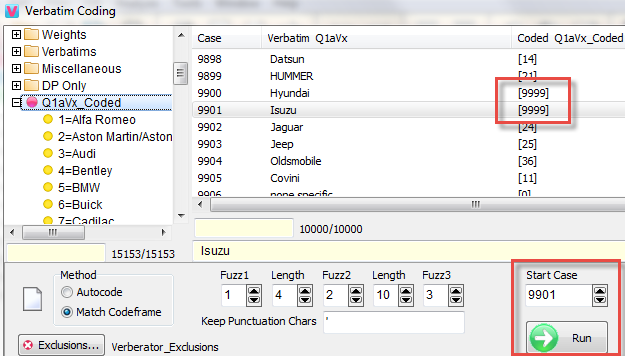
Edit cases 9900 and 9901 to be [9999] using the double-click method
Set StartCase to 9901
Click Run
Case#9901 is matched to the code frame as code 23, but case 9900 is untouched.
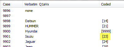
As a closer simulation of a tracking environment
Close Ruby to release all files
Open Q1aVx_Coded.cd in a text editor
Remove lines 9901/10000 and Save
Open Q1aVx_Coded.met in a text editor
Change Cases=10000 to Cases=9900
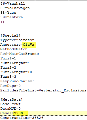
Note the ancestor is Q1aVx.
Save
Restart Ruby
Open the Verbatim Coding form
Double-click Q1aVx_Coded to load it
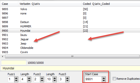
There are no codes for cases 9901/10000, but the verbatim text for those cases is known from the source variable Q1aVx.
Set StartCase to 9901
Run
The new cases only are coded.
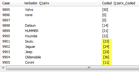
Check for miscodes and fix if needed, then Clean and Save as above.
The Memo Field
Sometimes the verbatim text can be too long to read. The selected verbatim is always in the scrollable Memo field.
There is a splitter bar to increase the height (and show more rows) if needed.
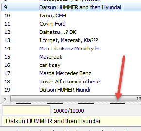
Edit Codeframe
Use this form to edit the reference master codeframe.
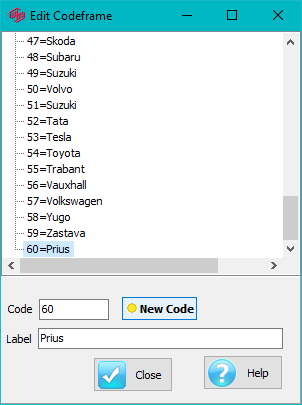
The form is accessed from here:
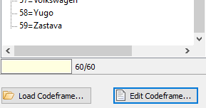
On Close, the Master codeframe is updated for any changes.
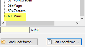
Existing items can be removed by the right mouse menu item Remove or by the delete key.
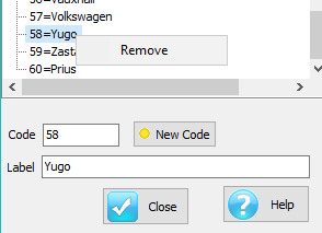
Metadata Group
Codeframes

Opens the CodeFrames Report form.
Cases per Variable

Runs a report to identify any issues with case counts in the active job.
Callouts
Opens the Edit Callouts form.
CodeFrames Report Form
Use the CodeFrames Report form to generate a report of all codeframes in the selected folder of the variable tree. If you do not select a folder then all variables will be processed. Frequency Counts can be included but that will take longer.
The report is written to a text file CodeFramesReport.txt and shown in Notepad. Output is tab-delimited for easy copy/paste to Excel.
This form is commonly used as a quick way to get holecounts.
The fields are saved with the job so they can be rerun at any time.
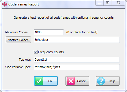
Highbound: limit each variable's report to this many codes - handy when large verbatims are present. Empty means no limit.
Vartree Folder: Branch of the Vartree to list - empty means all. Click the button to select from a form.
Frequency Counts: Run a table made from Totals and Side spec to show frequency counts.
Totals: The top axis of the table runs.
Side Variable Spec: The side axis of table runs. Blank means “*” - ie just all codes.
The side axis is made from each variable in turn with this field as its code range - e.g. Gender(tot;max;min;*;nes) then Region(tot;max;min;*;nes) etc.
Cases Report
This checks case counts in all variables reporting discrepancies, writes them to a text file CaseCountReport.txt and displays it in Notepad.
The Cases Report should always be run after an import to alert you to short variables (different case counts) etc.
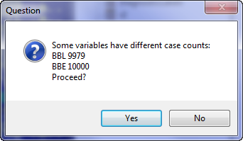
If you see the Some variables have different case counts: message it means there could be something wrong with the data:
the last update isn't complete
the data supplier provided an incomplete file
This recommends running the Cases Report to check if things need to be fixed.
A short variable means that table or construction will stop at the short number of cases and subsequent ones will not be included.
Callouts
The Callouts command exposes the Edit Callouts form to Analysts.
See Edit Callouts.
Archive Group
Zip

Opens the JobZip form:
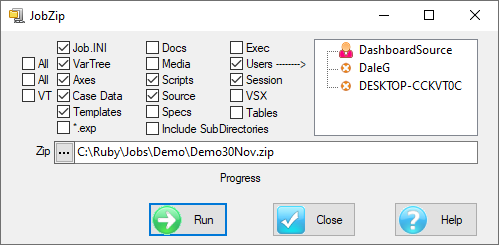
Use this form to archive (as *.zip) all or parts of a job. The zip file can be opened by Tools | Archive | Unzip. The advantage of this is that Ruby will handle all the details of which files go where. This is also the only way that job files can be uploaded to for Cadmium. The check boxes determine the archive content.
Job.ini: The job.ini file
VarTree: The currently selected variable tree. If All is also checked, then all *.vtr files in the job directory
Axes: The currently selected axes tree. If All is also checked, then all *.atr files in the job directory
Case Data: all files in the CaseData sub-directory
VT: Archive only variables which are in the current variable tree. This can dramatically reduce the size of the zip, but be aware that reports and constructions can reference variables not in the variable tree, so ensure that all reports still display, and that all constructions are up to date, before committing.
Templates: The template table, chart and specification, if present
*.exp: All case data export files, as a list of variables saved from DP | Tasks | Data Export
Docs: All files in the Docs sub-directory
Media: All media files in the Media sub-directory
Scripts: All files in the Scripts sub-directory
Source: All files in the Source sub-directory
Specs: All files in the Specs sub-directory
Include Subdirectories: All sub-directories of any selected directory
Exec: All reports under the Exec folder of the TOC
Users: All reports for the selected user folders
Session: All reports in the Session sub-directory
VSX: All files in the VSX sub-directory
Tables: Tables (*.cbt) are a table-only format (no charting) used to port Ruby tables to Carbon.
The default zip name is made from the job name and current date. You can change this to anything.
If there are security concerns, the *.zip can be password-protected.
Templates includes the templates cited on the Preferences Job Settings.
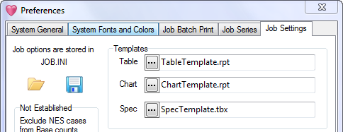
With the User checkbox ON you can select which users to include in the zip.
Unzip will replace those user folders with the ones in the zip.
You can use this to send a set of reports to someone.
Unzip

Unzip updates the job with files in a zip created by JobZip.
Ruby's Unzip is very fussy about the files it receives.
It must be created with JobZip, even though it is a standard zip file that you could make yourself.
There are many considerations in making the User section merge properly, so it is best to leave it to Ruby to manage the details.
Laser group
Laser: Provides direct access to on-line Laser jobs, using a proprietary no-frills browser. There is no connection between the current Ruby job and the Laser job(s), although most of the time your Ruby job would be the master job for the Laser deployment.
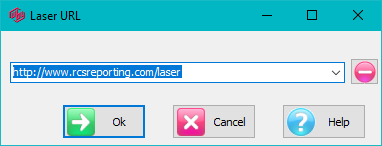
You can enter any server, or any URL for any web-page. Entries are remembered for the drop-down list, and can be removed using the red Minus button at the right.
The guest/guest login will always work for public jobs.
Dashboarder: This is a stand-alone executable which uses the same Excel-compatible (for the supported features) engine as Laser, and so can be used to design and test Laser dashboards without needing to upload first. It can also be used as a reporting extension on any Ruby job. You may prefer to do the design work in Excel as an already familiar environment. If so, open the XLSX file in Dashboarder before deploying to check for compatibility and alignment issues.
In the Ruby Demo job
Open DocsKPI.xlsx
Set the filters as Under 35, Male
Run
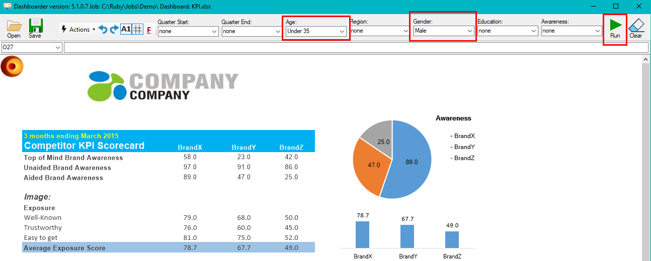
All tables and charts are repopulated with the filtered reports.
For details on how to set up a dashboard, see the online Laser help.
In short, you specify the filters on the sheet _Config_Filters, the Ruby reports which supply the dashboard's charts and tables on _Config_Reports, and use the sheet _Intermediate_Landings to do any other addition processing.

Sheets with a leading underscore are usually hidden before deployment.
Reports must be under a user name, here DashboardSource:
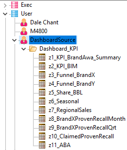
This is to isolate and protect the reports from other Ruby users.
Use the Actions menu for common tasks.
Check the A1 button to see the standard Excel row/column headers
Check the # button to see grid lines.
There are many custom hot-keys.
Control-M to merge the selected cells
Control-U to unmerge the selected cells
Control-F to show the Font dialog for the selected cells
Control-1/2/3 to align text left/centre/right
Control-4/5/6 to align text top/middle/bottom
Arrow keys to move the selected chart or shape
F1 to move the left edge to the left
F2 to move the left edge to the right
F7 to move the right edge to the left
F8 to move the right edge to the right
F9 to move the top edge down
F10 to move the top edge up
F11 to move the bottom edge down
F12 to move the bottom edge up
Home to snap the selected shape or chart to the nearest grid top-left corner
End to snap the selected shape or chart to the nearest grid bottom right corner
To quickly add data labels to a chart
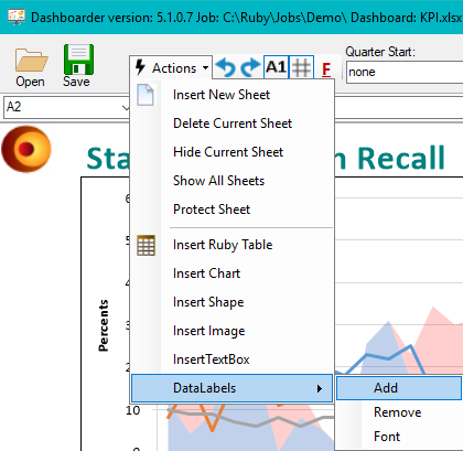
Enter a string of ones and zeroes
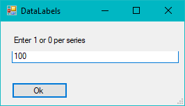
This will set data labels ON for the first series, and OFF for the next two:
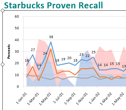
Analysis Tab
The Analysis tab is for advanced statistics.
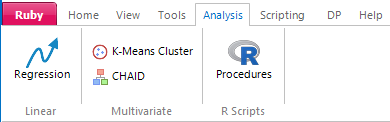
Linear Group:

Multivariate Group
R Scripts Group

Linear Group
Regression
This chart shows regression lines for each measure across three different sections of the X axis timeline.
Regression lines have the same colour as the series they represent.
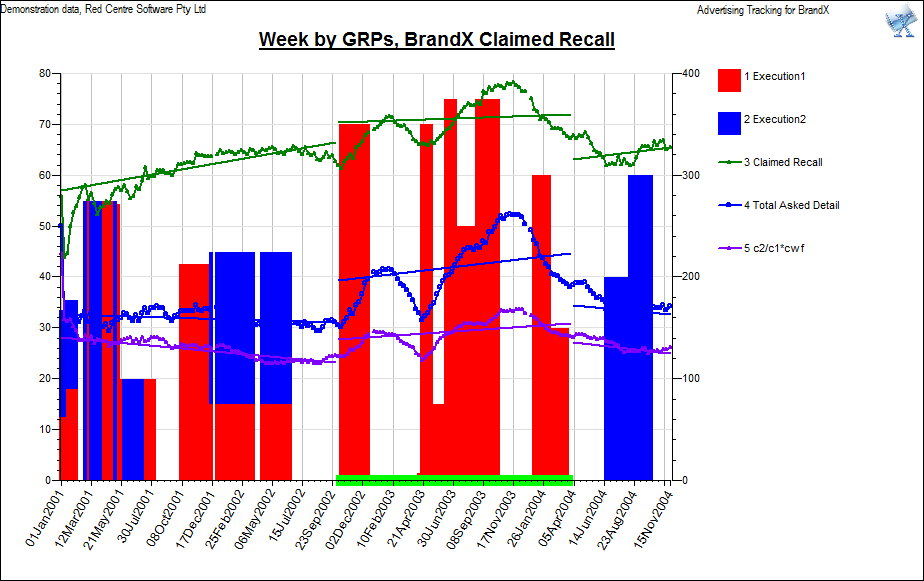
In this example there is one selection (green) on the X axis dividing the axis into three sections.
This selection is defined by double-clicking the left mouse button just above the horizontal axis and dragging out the required selection.
The trend line for a series is turned on or off via the right mouse context menu on the series legend, shown here:
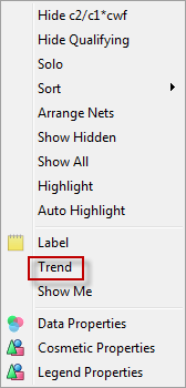
On the left of the Trend Line Regression form below, you select a series, in the middle you select a section, and the linear regression statistics are shown on the right.
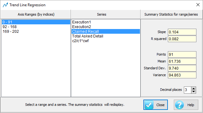
Slope: the slope of the trend in y units/x units
R squared: the coefficient of determination (the proportion of variance explained)
Points: the number of points in the range.
Mean: the mean over the range
Standard Dev: standard deviation over the range
Variance: variance over the range
Decimal places: set the number of decimal places displayed on the right panel
Multivariate Group
K-Means Cluster

Opens the Cluster Analysis form.
CHAID

Opens the CHAID - CHI-squared Automatic Interaction Detection form.
K-Means Clusters
The idea behind clustering is to find groups of cases that seem to be 'similar'.
All clustering techniques will have a 'distance' measure that gives a value to how 'similar' two cases are.
The most common is the 'Euclidean' distance that sees the case's responses as coordinates in a multidimensional space.
At any time each cluster will have a mean position in this space (hence the term k-means).
Each iteration involves seeing if any cases are closer to other means and swapping the cluster they are in.
After that the means are recalculated and the process continues till no cases swap.
Initialisation is fairly critical. Randomising is popular but can produce different results for different runs.
Ruby's initialisation distributes codes and values evenly across the clusters for a more stable result.
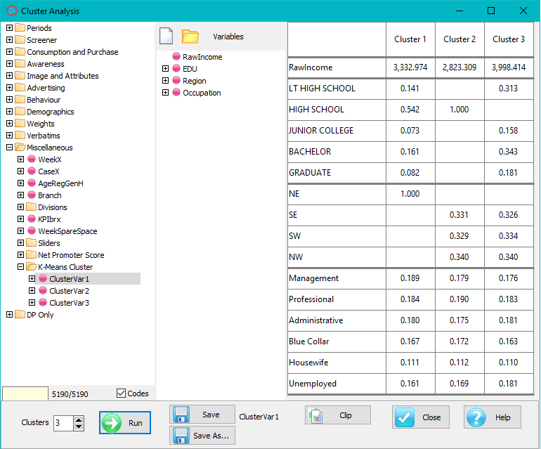
Cluster Icons and Their Functions
The left panel of the Cluster Form shows the familiar variable tree for the selected job.
The result of the analysis is a new Ruby variable that can be used like any other, so double clicking here will load an old analysis.
The middle panel holds the variables and codes that are the categories to be used for the distance measurement.
The right panel is a table showing the result of the run.
For uncoded variables it is the value for that mean
For coded variables it is the proportion of each code in the cluster
The bottom panel holds buttons for selecting a job, loading and saving cluster variables and running the analysis.
Exercise: Education and Income
In the Ruby Demo job, load ClusterVar1 (in the Miscellaneous folder) by double-click or, if not in your vartree, then by the File Open button at the top of the Cluster form.
Run
To build an analysis from scratch:
Drag variables RawIncome, EDU, Region and Occupation into the middle panel
Remove EDU(6) No Answer with the [Delete] key
Set the number of clusters to 3
Run
Save As MyClusterVar
What the result means
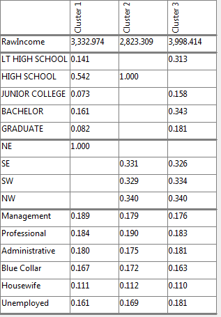
This table is the result of the above run. What you are looking for is good separation of the clusters.
Cluster 2 has 1.000 against High School meaning all its cases had that code.
Cluster 1 has 1.000 against NE and a majority 0.542 (54%) against High School.
The RawIncome variable doesn't seem to be showing much separation with about 3000-4000 as the mean of each cluster.
The Occupation variable also shows not much separation.
So you might say Cluster1 is mostly High School in the NE, Cluster2 is High School, and Cluster3 is not really well defined at all.
You can change things and run the analysis again looking for a good result before committing with a Save.
You can remove codes/variables you don't think are distinguishing, you can change the number of clusters, and you can change the order of the variables.
Initialisation is critical and that will be changed by variable order.
Swap Region and EDU
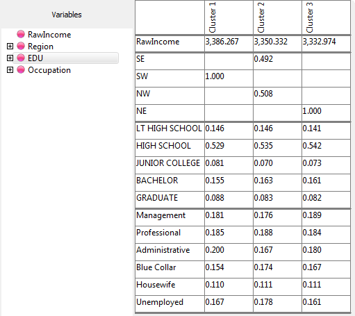
Swapping the order of variables will change initialisation possibly resulting in a different outcome.
Here, by moving Region above EDU ([Ctrl]-[UpArrow]), Cluster 3 now looks well defined.
This is largely tinkering at the edges and the differences won't often be large.
Changing cluster number will have the biggest effect.
Change Cluster Number to 4
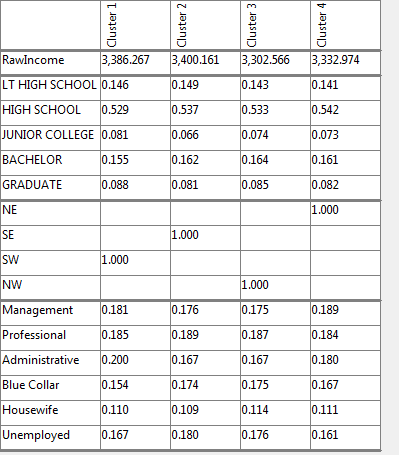
This is the result for 4 clusters. Notice Region is now the strongest distinguisher with the clusters now each having only one region code exclusively.
This is to be expected in the Demo job since most variables are random - not useful really.
The EDU/Income variables in the Demo job are actually real data from the General Social Survey (GSS) so reducing the influence of the random variables should produce some credible results.
Remove Occupation
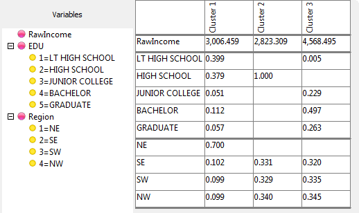
Removing the Occupation variable from the original setup, even with 3 clusters, has a good effect.
RawIncome is now a good distinguisher showing Cluster 2 low and Cluster 3 high.
EDU is distinguishing with Cluster 2 all High School, Cluster 1 mostly in low (0.399, 0.379) education categories and Cluster 3 mostly in high education categories (0.497, 0.263).
Once you find a result that appears to have meaning use the Save buttons to commit it to a variable. You can always reload the variable here to change things later.
Initialising Clusters
Here are some details on how the clusters are initialised.
MyClusterVar above looks like this after initialisation:
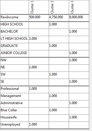
For the uncoded variable RawIncome, the means start off evenly distributed across the range.
For the coded variables the codes are sorted by base size then 1s are diagonally distributed across the clusters, starting at the next cluster for each subsequent variable.
The RawIncome var starts with Cluster1,
The EDU variable starts with cluster2 and you can see the diagonal line of 1s wrapping around
The Region variable starts with Cluster 3 and again wraps around diagonally ... etc.
This ensures clusters get an even share of big codes and variables get an even share of clusters to start off with, plus the initial means start off well separated.
When the run finishes, the decimals in the code cells are where the mean is for that coordinate.
e.g. The final 0.542 for HighSchool Cluster1 means a case with 1 for HighSchool is 1-0.542=0.458 away from the mean (for that coordinate).
CHAID
CHAID stands for Chi Square Automatic Interaction Detection.
CHAID shows interactions between a Dependent variable and any number of Independent variables. For an explanation of how CHAID works see here.
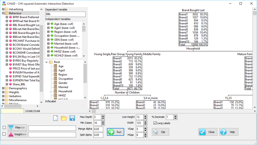
The left panel shows the familiar variable tree for the selected job.
The middle panel top section is the drop zone for Dependent and Independent variables dragged from the left.
The middle panel bottom section shows all the tables that have been run.
Click on any of these to see some information at the bottom of the middle panel.
This also shows the table in the right panel - click on a folder node to return to the CHAID display.
The right panel is the visual representation of the CHAID tree. Only successful candidates from the table set are shown here.
The bottom panel holds buttons for loading and saving CHAID specifications (.rch file), running the analysis, display controls and clipping.
Exercise: CHAID Analysis
This example creates BBL.rch. Alternatively, open this file
 from the Ruby Demo job.
Specify an analysis
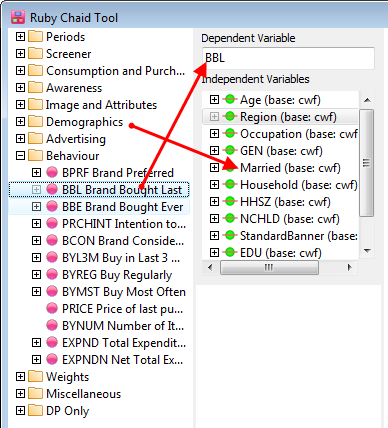
Drag BBL into the Dependent Variable
Drag the Demographics folder into the Independent Variables
NB: Not all demographics are suitable for CHAID analysis. Standard Banner is a constructed variable whose codes are not independent.
Remove StandardBanner and RawIncome by selecting them and pressing [Delete]
Identify Nominal variables
Most variables have codes in a meaningful sequence but Region should be identified as Nominal.
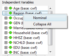
Right click on Region and select Nominal
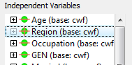
The icon changes to indicate this variable is Nominal. This means any pair of codes could be merged. An ordinal variable only allows adjacent codes to be merged.
Run
Click Run

During processing the status bar shows what tables are being generated.
Display
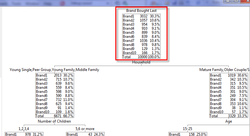
The result is a list of tables and a CHAID tree.
The display starts at the top showing the distribution of codes in the dependent variable (Brand Bought Last).
Underneath that are successive splits.
The first here is the Household variable that showed the lowest p value after its codes were merged into two sets.
The boxes show the distribution of BBL codes after the split.
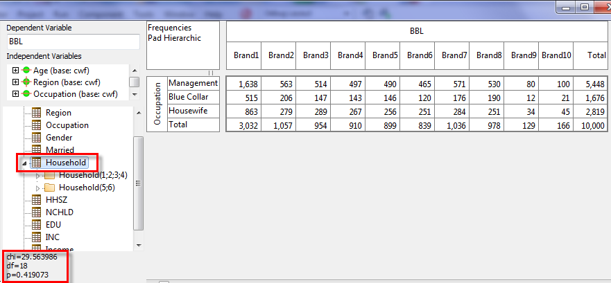
You can see the actual table by clicking on the Household node in the tree. This also shows the test results for that table.
The Household node has branches under it showing subsequent splits. You can click on any of the other tables to see its test information as well.
Click on any folder node to return to the CHAID display.
Scroll to the bottom.
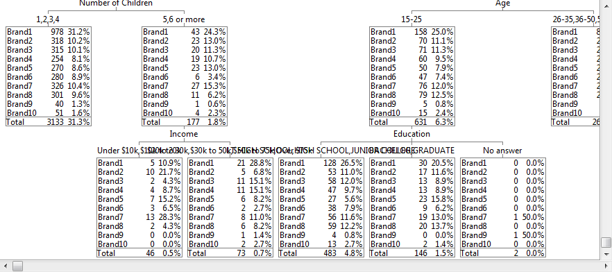
The code label sets are overlapping. You can switch to short labels (as just the codes) for a cleaner display.
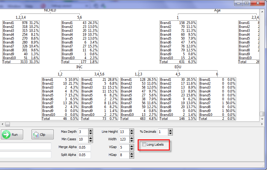
Variables now appear as their name rather than description and codes as their value rather than description.
Removing codes
Notice at the bottom of the display EDU(6) only covers two cases. You can remove this node and rerun.
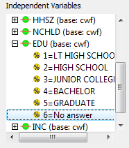
Open the EDU variable and [Delete] code 6
Click Run
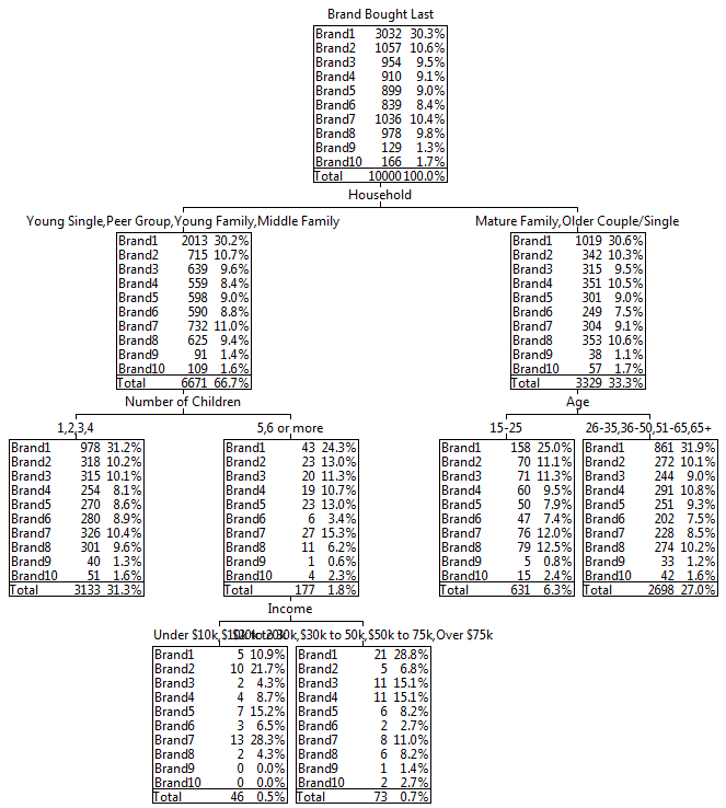
The resulting table shows the categories that were significantly different in their relationship to the BBL variable.
You can use the controls at the bottom to change the display.
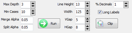
Max Depth: limits the depth of the tree. A greater number means more nodes and will take longer.
NB: Each depth level is a variable split and actually creates two layers in the visible tree - one for the variable and one for its categories.
MinCases: the threshold case count for a merged row to be a candidate for the next split.
MergeAlpha: the threshold p value for merging two rows in a table.
Any pair of rows whose Chi Square p value is greater than this are considered not significantly different so will be merged.
Increase this to reduce the degree of merging.
SplitAlpha: the threshold p value for splitting a variable and making new nodes for each of its categories.
Any table whose adjusted Chi Square p value is greater than this is considered not significant so is not a candidate for splitting.
At each node only the table with the smallest value is actually split.
Line Height: the pixel height of text lines in the CHAID tree.
Width: the pixel width of the boxes in the CHAID tree.
VGap: the vertical gap between boxes and labels.
HGap: the horizontal gap between boxes.
%Decimals: the number of decimals for the percent column in boxes
Long Labels: switches between diagnostic and expanded labels.
All of these settings are saved in the .rch file.
You can define the filter/weight and turn them on/off with the check box for a different Run.
These are also saved in the .rch file.
How CHAID Works
CHAID it is a recursive process involving alternating Merging and Splitting stages using Chi Square calculations at each stage to identify significant relationships.
Merging
Each candidate Independent Variable is examined to see if any of its codes are sufficiently similar against the Independent Variable to warrant merging.
This involves checking a small table with just two code rows against the Dependent Variable.
If the Chi Square p value of this is greater than a MergeAlpha reference value the codes are considered mergeable.
The pair of codes with the greatest p value is merged and the process repeated with the now smaller variable table.
This stops when no pairs are mergeable or the variable is reduced to two categories.
Variables can be Nominal, meaning any pair of codes can be merged; or Ordinal, meaning only adjacent pairs of codes can be merged.
A rating scale would be Ordinal because the codes have a meaningful sequence. A geographic location variable would probably be Nominal.
Splitting
All Dependent Variables (most now with fewer categories than codes) are crosstabbed against the Independent Variable.
A Chi Square test is done on the resulting table and any that give a p value less than a SplitAlpha reference value are candidates for splitting.
The candidate with the lowest p value is split.
If the table has merged rows its p value is multiplied by a Bonferroni adjustment.
This is essentially the number of ways the original set of categories can be merged into the resulting set.
Because of this, displayed p values can often be greater than 1.
The tree grows a node for the variable and each of its categories makes a child node. Under each of these the process is begun again with the remaining variables.
Recursion
Under each split node a new set of tables for any remaining variables are run against the Dependent Variable, now filtered to the chain of category splits that lead to this node.
Each of these tables is again checked for Merging and the resultant set checked for Splitting.
The process stops when no candidates for splitting are available, or when a Maximum Depth has been reached.
R Scripts Group
This runs a VB script which uses the current table as the input to the selected R procedure. The form design is exposed for review in RubyRun_RScripts.vbs. If you want to call your own R routines, start with Run_RScripts_Template.vbs.
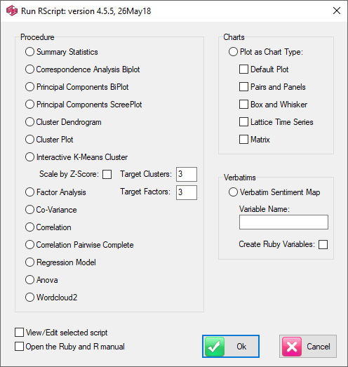
Procedure: the R script to apply to the current table
View/Edit: view and edit the R script for the selected procedure.
See Help | Documents | Ruby and R.pdf for full details on the supplied R scripts, and how to extend for your own custom procedures.
Scripting Tab
Riut5ine tasks or complex procedures can be scripted in VBScript (*.vbs), VBA (via MS Office applications), JScript (*.js), VB.Net (.vb), C#.Net (*.cs) or any other language platform which supports Windows COM (Common Object Model).
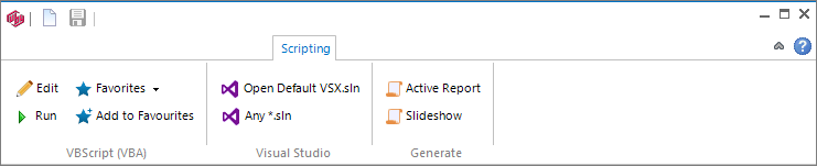
The most common languages used for Ruby scripting are VBScript and VB.Net. These are the most accessible languages for non-professional programmers (simplest syntax, generally readable). Libraries in VBScript and parallel VB.Net to simplify many tasks are in the Ruby subdirectory, as Ruby*Library.vbs and Ruby*Library.vb. There are many example scripts in the standard Ruby installation.
The Scripting tab gives access to both the inbuilt VBScript engine and the full Visual Studio for more advanced projects.
The following scripts use VBScript and are based around the Demo job:
Standard Tables Script
Standard Charts Script
See Also: Statistics Scripts
VBScript (VBA) Group:
Visual Studio Group:
Generate Group:
VBScript (VBA) Group
 Open the inbuilt VBScript (and JScript) editor.
 Run a VBScript (or JScript) without opening it first.
 A user-specified list of regularly used scripts.
 Add a selected script to the Favorites list
VBA (Visual Basic for Applications) is the MS Office macro language. VBA syntax is almost identical to VBScript.
Standard Tables Script
Most continuous jobs have at least one set of tables that is run regularly.
You could simply specify each of the tables in the set manually, organise them into a folder in the TOC, and then update just this folder.
But if you want to run by different period files, or different weights, or apply a global filter, then it is tedious to have to make the same change to many manual specifications.
Where a table set needs to be run frequently under different periods, filters or weights, a better approach is to commit the entire run to a script.
There is a demonstration script GenerateStandardTables.vbs in the Demo job.
To run this script go Scripting|VBScript|Run, select it and click on Open.
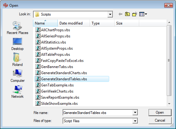
Eighteen tables are generated and displayed in child windows.
These folders and tables in the Demo job were created from this script:
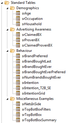
Standard Charts Script
The standard charts for a job are specified and generated in much the same way as for tables, but since more parameters are required, the calls to Process() and the Process() sub-routine itself are different.
There is a demonstration script in the Demo job called GenerateStandardCharts.vbs.
To run this script go Scripting|VBScript|Run, then select and open GenerateStandardCharts.vbs.

Eighteen charts are generated and displayed in child windows.
These folders and charts in the Demo job were created from this script:
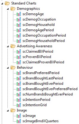
Using the Script Editor
Ruby has a built-in script editor, accessed via the Edit button on the Scripting tab of the Ribbon:
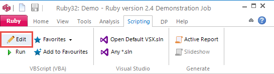
Script Editor Window
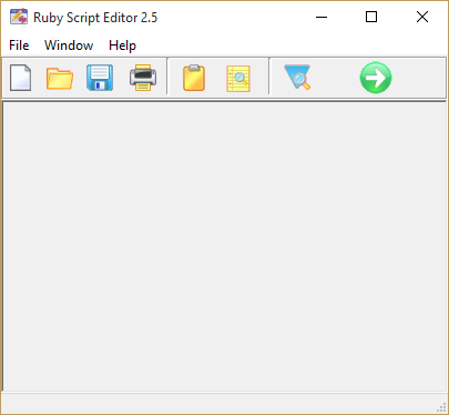
File Menu
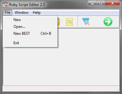
New: Opens a blank AutoEditForm document for you to begin writing your script in VBScript or JScript.
Open: Opens an existing script.
New BEST (Ctrl+B): Opens a new AutoEditForm document with a skeleton VBScript ready for you to insert your code.
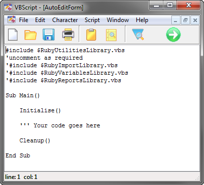
File Menu when a file is open
The File Menu changes when a file is open to contain standard application, file and print commands:
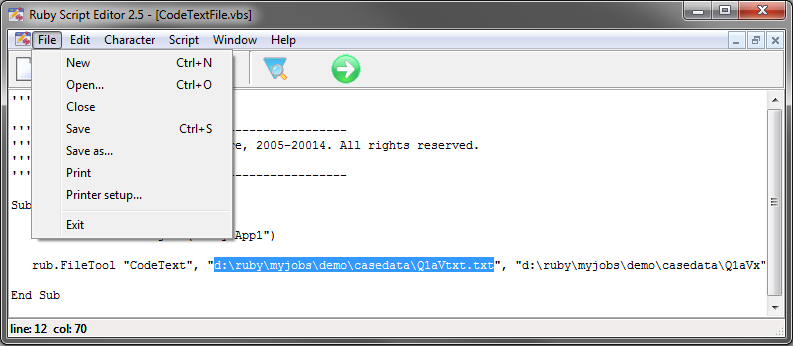
Edit Menu:
The Edit Menu also contains standard commands:
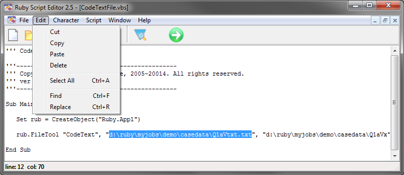
Character Menu:
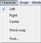
Left: Left justifies text
Right: Right justifies text
Centre: Centres text
Word Wrap: Toggles word wrap off and on
Font: Allows choice of font name, style, size and colour
Script Menu:
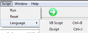
Run: Runs the script in its native environment (VBScript or JScript) - same as green toolbar icon

Reset: Resets the scripting environment after a script has failed to run
Language: Sets the language used to program the script to either VBScript (Ctrl+B) or JScript (Ctrl+J)
Window Menu: The Window Menu contains standard window functions.
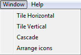
Help Menu:
The Reference link in the Help Menu opens the RubyAPI.chm document.
The RubyAPI.chm is the programming reference for Ruby Automation via VBScript and VB.Net using our custom API calls and libraries of commonly used function calls.
Script Editor Toolbar

The icons (from left to right) are as follows:
New, Open, Save, Print, Clipboard, Print Preview, Search, Run
Note that the current cursor position is shown at the bottom left of screen:
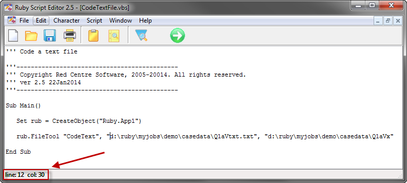
Visual Studio Group
 Open the default Visual Studio project for the current job. This is expected to be in the sub-directory vsx.
 Use the second button to open a different project.
Generate Group
Generate the specification script for reports and show in the default text editor (usually Notepad.exe).
 This converts the current report to its syntax form in the language specified on the System General tab of the Preferences form.
 This converts the current slideshow to its syntax form in the language specified on the System General tab of the Preferences form.
The generation is of the specification only. To run, you need to copy/paste to your script.
See also Generate Spec.
DP Tab
The DP Tab is the central point for DP to set up and manage jobs.
You can import case data, build or modify codeframes, construct new variables, modify the variable tree, maintain named code lists, add or modify callouts and events, run several utilities, set some job and system preferences, update all constructions or any existing reports with new data, and upload/download jobs or job sections to a cloud storage customer account.
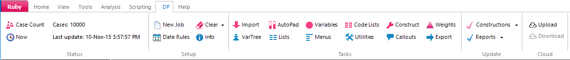
See Job Setup - Ad Hoc and Trackers, Job Update, and follow the links below for help on the controls and commands in the DP tab groups.
Status Group:
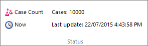
Setup Group:
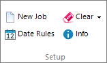
Tasks Group:
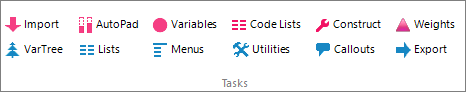
Update Group:
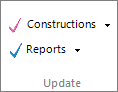
Cloud Group:

Status Group
The Status Group shows the number of cases in the job and the last time a data update was run.
Case Count

Count cases for the first variable in the variable tree. If there is no variable tree, the first .CD file found in the CaseData directory is used instead.
Now

Set the date of last update to the current date and time. You might do this to provoke all charts, tables and constructed variables to be regenerated. When any table or chart is opened or a constructed variable is used, the internal date is checked against the date shown here.
Setup Group
The Setup group shows the current job name and location, and is where to start when creating a new job.
New Job

Opens the New Job form.
Date Rules

Opens the Date Rules form.
See also: Handling Dates.
Clear

WARNING: Be very careful - this is a dangerous operation.
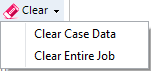
Clearing can be useful when you are setting up a new job, trying various import strategies, and you have to frequently start again.
Select from the dropdown menu to clear either the Case Data only or the Entire Job.
Clear Case Data: Remove all case data from the *.cd files only, keeping all metadata and other job files
Clear Entire Job: This clears the CaseData directory, the Axes (in the Specs folder), the axes tree (in the job's root folder) the Vartree and sets Cases to zero. Reports are not removed.
A backup of the CD, MET, VTR, ATR, AXS, TBX and INI files is made in a directory under the job.
Successive backups will be named backup1, backup2 etc.
If you want to undo a clear, you will have to manually copy the VTR, ATR and INI files back to the job folder, the AXS and TBX files to the Specs folder and the CD and MET files back to the CaseData directory from the backup folder.
Info

Opens the Job Information form.
New Job Form

Creates the sub-directory structure and initial default files for a new job.
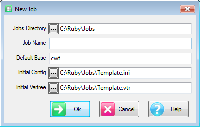
Jobs Directory: The parent directory for this job and others you may want to consider as a group of jobs
Job Name: A job name can be any legal subdirectory, however it should start with a letter, and have no apostrophes, and no punctuation characters other than underscore or hypen
Default Base: This base will be applied to new variables as they are created either at import or on the Variables and Construct forms. The default base is usually cwf (Cases Weighted Filtered) but can be any of the allowable bases.
Initial Config and Initial Vartree: Use these fields to copy pre-existing *.ini and *.vtr files as job.ini and vartree.vtr to your new job. This allows you to apply house standards or pre-configured settings appropriate to classes of jobs. This can save a great deal of time when setting up a new job which is similar to others. Leave the fields blank to use the Ruby defaults.
OK: On clicking OK the job is created and entered.
Date Rules Form
Use the settings on the Date Rules form to resolve ambiguities when reading a date string.
These do not affect how dates are displayed.
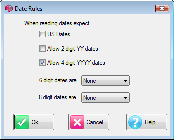
When Ruby starts up, a check is made with your computer to see if you are using USA dates and this switch is set to match.
The setting is saved in Job.INI so any job can override it.
Ruby has to convert text to dates in two main places:
When a date variable is being read in (all its code labels must be valid date strings)
When attempting to guess data types during an import
There are other places like the start date on the Date Constructor form.
Ruby reads dates by separating the string into up to three sections that are each either all numeric or all alphabetic.
Anything else is regarded as a separator so 12Jun2005, 12 Jun 2005, 12/Jun/2005 and 12*-()Jun%^&2005 will all be recognised.
If the three sections are all numeric, Ruby needs to know whether to read e.g. 12 6 2005 in US or European format.
When there is only one section that is all numeric Ruby needs to know how to interpret 2, 4, 6 or 8 digit strings.
Otherwise reasonable variation is tolerated - for example June 12, 05 is not ambiguous.
When the year part is only two digits Ruby assumes it is between 1950 and 2049.
It is best to start with all settings off and turn them on only if ambiguities are encountered.
See also: Handling Dates.
Job Information Form
The Job Information Form shows information about the job and is where you can edit and save the job description.
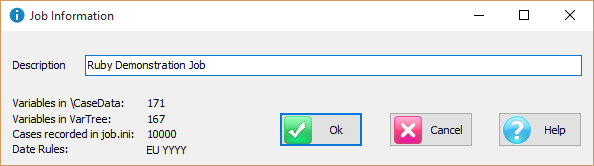
Tasks Group
The items in the Tasks Group, from left to right, follow the usual sequence for updating a job.
Import

Opens the Import Data form.
AutoPad

Pad short variables (usually because they have been dropped from data collection) with empty cases. See AutoPad
Variables

Opens the Edit Variable form.
Code Lists

Opens the Code Lists form.
Construct

Opens the Construct Variables form.
Weights

Opens the Weights form.
VarTree

Opens the Edit Variable Tree form.
Lists

Opens the Lists form.
Menus

Opens the Edit Custom Menus form.
Utilities

Opens the Utilities form.
Callouts
Opens the Edit Callouts form.
Export

Opens the Data Export form.
Import Data Form
The
button on the Tasks group of the DP tab opens the Import Data form: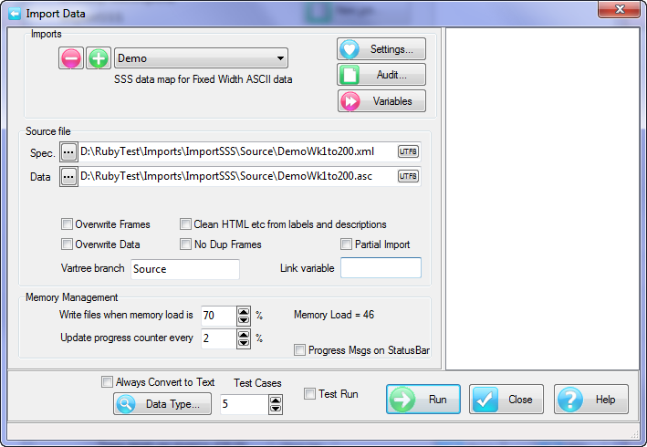
Imports
The source data for a job can be imported from a variety of sources - for example the main data comes from a card image file and some secondary data comes from Delimited ASCII out of Excel. Each import is user-named and recorded in job.ini in case the job ever needs to be rebuilt from scratch.
The drop down list shows all the imports so far.

 The plus and minus buttons are for creating a new import or removing the current one.
 Clicking
opens this form: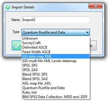
You give the import a name for later identification and select the import file type from the Type drop down.
The different formats need varying degrees of attention at import time. Some formats are well formed and require no preparation before running the import but for most there is usually something to check.
If the data comes in waves, the first import and subsequent waves also have different things that need to be considered, such as how the variables from one wave are matched with those from previous waves. Some formats have reliable names, some reliable descriptions and some have nothing reliable. See the Test Import form later for further details.
 Some imports have settings that can be edited here.
 All imports after the first will have an Audit file (an exhaustive listing of all differences) that can be viewed here.
Source File
All imports have a data file. Some import types also have a specification file that describes the variables, their codeframes and other information. Other types have this information incorporated into a single data file. You can use the browse buttons to select the files or type the names straight in. It is best if all source files are in the job's Source directory. If you select files outside the Job's directories Ruby will offer to copy the file into the Job's Source directory.
Overwrite Frames: For a job that has data arriving in waves it is usual to completely overwrite the code frames at each update. This would be a good idea if the data source could be relied upon to always have the latest complete set of codeframes and labels (e.g. SAVs or SSS). With Overwrite Frames OFF the codeframes are simply updated with any new information - new codes or new labels for old codes, with new codes being added at the end of the existing code frame, regardless of numeric order.
Overwrite Data: You might want to Overwrite Data if you are repeating the imports for some reason and want to start from scratch. Normally this switch would be off so that new data is appended to existing data.
Clean HTML: Some data sources keep html tags and questionnaire deployment information in labels and descriptions. e.g.
q1 = Choice of Holiday
code1 = Queensland
With this switch ON anything inside the <> brackets is removed, thereby producing clean labels.
No Dup Frames: Some imports have one codeframe shared by a number of variables, which normally come into Ruby as Dup references. Sometimes you don't want this. With this switch ON the import will copy the codeframe rather than making a dup reference.
VarTree Branch: This identifies a branch of the variable tree under which new variables should be added. This keeps them in a convenient place and makes it easier to organise your tree. If the branch does not exist it is added to the end of the tree. If Vartree Branch is blank new variables will be added to the end of the tree. If there is more than one folder of this name, the first is used.
Partial Import, Link Variable: Sometimes the data for a wave comes from a number of sources. If you have already imported the main body of data for a wave but there are some variables in a separate file, then that is a Partial Import. You need to identify a Link Variable that exists in both the job and the second data file so that data can be matched to the right case. When the import runs it expects all variables involved (except the link one) to be short by the same amount and extends them by adding data for available cases and blanks for those cases not in the file. The partial import process creates .err where unmatched links are listed. This file can be viewed with any text editor.
Always Convert to Text: Some formats, e.g. SurveyCraft, can look for text variables that have not been identified as such up front and result in a sequence of Convert? questions.
Set this switch ON to automatically answer Yes to all these.
If you know there are no other candidates that will trigger the question (e.g. potential dates variables) you can expedite the import by asserting Yes to all the convert questions.
Test Run: If you only want to import a few cases for a test set this Switch ON and set the number of cases in the thumbwheel.
Memory Management
Windows does a good job of managing memory but if you run too close to the limits then time is wasted as Windows goes back and forth to its swap file. For large imports it is a good idea to have the data written away periodically so that memory can be retrieved, thereby relieving the pressure on Windows. As the import progresses the memory load is reported as a percentage. You can set the percentage at which Ruby should stop reading, store what it has, and retrieve memory. With experience you will find what suits your system best.
There are two considerations in deciding the threshold:
1. The maximum figure the operating system will tolerate before using swap files.
In Win10 this is roughly 80%, while for Windows 7 it is about 70%
2. The minimum figure to protect resources.
For 32 bit Ruby Windows will give it no more than 2 Gb of RAM.
If you allow Ruby to access more memory than 2 Gb, you will get a memory exception error.
You should leave a bit of memory headroom as well, so an example calculation for an 8 Gb machine might go like this:
...Let Ruby use 1.8 Gb
...What percentage of 8 Gb is 1.8 Gb? 1.8/8 * 100 = 22.5%
...This tells you to set your memory maximum at about 20% more than the current memory load.
(i.e. If the current memory load is 36% then set the threshold to 56%)
For 64 bit Ruby you should rarely have to bother since Windows allows 64 bit programs to access all RAM.
Vertical Read: Some import types can be read vertically or horizontally and often one way will be quicker than the other. For instance, a delimited ASCII file presumes that the first row comprises the variable names and that every subsequent row is a case of data. Reading this vertically is usually kinder on memory because it reads one column at a time as a single variable and then writes it to disk before starting on the next column. Reading horizontally builds every variable's data progressively in parallel and might have to stop periodically due to memory load. Once again, experience will tell you which way is better for any import file.
Progress Msgs on Status Bar: Normally messages are displayed in the progress list on the right. This can contribute often substantially to the import time. You can save time by diverting them to the Status Bar.
Data Type
This opens the Import Data Types form for examining the first few cases of data and to identify data types.
For formats that include information about the type of data you probably will not need this button.
For some formats, you will need to check data types at the first import but at most other times you can probably run without testing.
Run
On clicking Run the import process executes. Progress is indicated by the counter in the status bar and by messages appearing in the panel on the right.
These might be the names of variables as they are processed or significant steps in the import.
Checking Test Run limits the import to the first few cases (here 5).
If a source variable name begins with a Ruby three-letter + underscore function name, eg var_01 or sum_Units, then it prefixed with 'rn_' for 'renamed', as rn_var_01 and rn_sum_Units.
Data Types Form
The Data Type button on the Import form opens the Data Types form.
This form shows the first N cases in a test grid (N comes from 
The left column shows all the variables in a scrollable list. Double-click on a variable to shift the grid display to that one.
The icons indicate the Data and Code types currently set for the variable.
On the key below, 0 means unknown, 1 means Text/Build, 2-5 mean Number (Unknown, Build, Spec, Self) and 6-9 mean Date (Unknown, Build, Spec, Self).
Variable names appear across the top and the first five rows show the data for the first five cases.
MET Type: is the data type currently stored in the variable's .MET file
Data Type: is the type that will be stored in the .MET file when you click Write Met
Code Type: tells Ruby how the codeframe labels will be made
Click column label for codeframe
Some imports supply the codeframes in a spec file and this can be very helpful in deciding what types to assign.
Right-click on the grey column header to see the variable name, description and codeframe so far.
Click the Expand button to see Duplicate and Self codes expanded.
Data Types
This simply indicates what sort of text to expect when the variable's data is read in.
Ruby's .CD data files can only contain numbers and a few special characters so non-numeric input has to be converted to a code immediately.
Text data is stored in the codeframe as a label and its code number is stored in the .CD file.
Date data is converted into an internal numeric representation which is stored in the .CD file.
Numeric data can be stored directly in the .CD file.
Code Types
This tells Ruby how the codeframe labels will be made.
Spec: Sometimes the labels are provided directly by the Specification file which accompanies the Data file.
For other imports you may intend writing the code labels yourself in the Edit Variable form.
Either way, Ruby doesn't need to do any generating of codeframes at import time.
This usually means the data will come in as numbers.
Build: Data that comes in as alpha text has to be given a code number as it is imported, meaning that the text itself is immediately stored as a code label.
Ruby builds the codeframe dynamically and assigns code numbers to unique text strings.
Each new batch of labels is sorted alphabetically but is not mixed with the labels from the previous import; otherwise code numbers assigned at the previous update would change. Date data is an exception to this because the number stored in the .CD is an actual date number, not a code reference, so codeframes for date variables are completely resorted after import to ensure they are in chronological order and may change code number.
Self: Variables with quantitative numeric data can be flagged as self-coding.
The data is stored in .CD files but the actual codeframe is generated dynamically when the variable is used.
Guess Data Types
Ruby looks at the data read in for the first five cases and makes a guess at the type.
If the five cases can all be interpreted as a date then Date type is assigned, if they are all numeric then Number type, otherwise Text type.
Text data can only be Build-codeframe code types but the others could be anything.
To change Data Type or Code Type, left-click on a cell and select from the popup that appears.
For Date and Self (coding) variables you can set specific details here.
This can also be done later using the Edit Variables form.
For regular date data you can specify the cycle details by right-clicking on the green date cell.
This presents the Date Cycle form.
For Self Coding codeframes you can specify the style of generation by right-clicking on the blue Self cell.
This presents the Self Code form.
Self-coding generates the codeframe by one of three methods.
Bands: The data is divided into a number of equal size bands between highest and lowest value.
If the lowest value is close to zero, Ruby uses zero as the lowest.
Steps: The data is divided into equal sized steps, as many as are needed to cover lowest to highest.
Again, if the lowest value is close to zero Ruby uses zero as the lowest.
All: Each unique value in the data becomes its own code.
Importing SurveyCraft
SurveyCraft imports use a SurveyCraft .PRN file (of the binary .SPC) as the Spec and .SEQ as the Data.
Method
SurveyCraft can store text data but doesn't distinguish between that and numeric data without a codeframe - both are called Uncoded - so you will probably need to tell Ruby which is which.
After doing this make sure no variables have been wrongly identified as Date types - if you have four-digit-dates ON you may find a Postcode variable has been identified as date.
There are a few settings you should check in the Settings form.
SQDigits:
PRN files are column organised with descriptions and other details in particular columns that are different depending on whether the original SurveyCraft data had three or four digit SQ numbers.
If you don't know this, check the PRN file. Question descriptions start in column 27 for four digit and 22 for three digit files.
Header lines:
PRN files have a page header inserted following a new page character.
These usually cover three lines but you should check the PRN file - sometimes they take four.
Generally it doesn't matter, but if the page break occurs in places like range descriptions it can cause misreading if the right number of lines is not skipped.
Variable leading char:
SurveyCraft variables are always Q followed by a number.
Ruby preserves the number but you can change the leading character to anything else.
It is a good idea to do this because questionnaire references are also usually Q followed by a number so using a different leading character for variables helps to avoid confusion.
Looped frame leading char:
Ruby recognises R specs in the PRN file that describe SurveyCraft looped variables and which create Ruby hierarchic variables.
For instance, using the settings above, R 172 173 will produce a Ruby hierarchic variable named s172s173 with two levels named p172 and p173.
Earlier in the import Ruby probably will have imported the single variables Q172 and Q173 as s172 and s173, so to avoid confusion a different letter is used for the codeframes of the hierarchic variable.
Include SC arithmetic and skip codes:
SurveyCraft specs can include interview instructions, internal constructions and other things that appear as codes like
C0 =S
C1 =W6
C2 =1+2
With this switch ON these will be added to the codeframe as is and you can decide what to do with them in the Edit Variable form.
With this switch OFF these codes are ignored.
Importing SPSS .SAV
SAV files have the descriptions, labels and data in a single file.
Data and code types are inferred from other information in the file, so while you can use the Import Test form to inspect the data before import, you cannot change any variable types.
Alpha codeframes like...
alb = Albania
blg = Belgium
...are recognised and converted to numerics in Ruby Variables.
No Dup(licate) Frames
Variables in SPSS often have common codeframes - typically the sets of variables that will be blended (Q1_1, Q1_2 Q1_3 etc.).
Normally Ruby imports these with Dup codeframes but that means you have to retain the source variables because the first is the only one with the actual frame.
This switch forces all codeframes to be explicit so you can use KeepSource=0 in blend files.
Ansi/UTF8
The ANSI button can be toggled to UTF8.
It only makes a difference for non-Latin alphabets except that apostrophes and some other punctuations characters come in several different forms.
One ANSI apostrophe character hex 92 is represented by a string of three characters in UTF8: hex E2 80 99.
If your punctuation looks odd, it could be the other type.
Missing/Invalid
The Settings form has one switch and a substitution character.
Remove Missing Codes: A SAV question with 777 identified as Missing will produce a Ruby CD file with 777s in it but the MET file will not have a code 777. This way the data remains and will be identified as Not Established in Ruby tables.
Replace Invalid: SPSS variable names can include many characters that are illegal in Ruby - e.g. because they are recognised as arithmetic operators. When illegal characters are encountered they are replaced (typically) by an underscore. So Q3$A in SPSS becomes Q3_A in Ruby.
We have seen a case where the SPSS included both Q1_1 and Q1.1 with the unfortunate consequence that when Q1.1 is converted to Q1_1 it collides with the actual Q1_1.
To avoid this, you can supply a different character to use to replace illegal ones - eq 'p'. Then Q1.1 becomes Q1p1 and doesn't conflict with Q1_1.
Method
You don't need the [Data Type] button. You can run the import immediately.
Using a Blend File
SPSS files often include lots of dichotomous variables that you have to construct up into single multi-response or hierarchies in Ruby.
Using a Blend file, you can do this at import time, typically reducing the variable count by over 90% for significant jobs.
See Blend Imports.
Importing Delimited ASCII Data
The simplest data files are self-contained ASCII files where the first row comprises the names of the variables and each row after that is the data for one case.
Some rows may be comments indicated by a special first character.
Some rows may even be short. A line with too few data items implies the last ones are missing.
These imports only have a data file but there are a few settings under the Spec button to facilitate variations.
The UTF8 button can be toggled to ANSI.
It only makes a difference for non-Latin alphabets except that apostrophes and some other punctuations characters come in several different forms.
One ANSI apostrophe character hex 92 is represented by a string of three characters in UTF8: hex E2 80 99.
If your punctuation looks odd, it could be the other type.
Click on Settings 
Delimiter: Select the delimiter character from the drop down list.
First Line is Variable Names: Generally, the first line of delimited data is the variable names but sometimes it is absent.
Use this switch to tell Ruby how to handle the first line.
Comment: Type in the character that indicates a line is a comment.
Missing: Sometimes these files have a special character like '*' to indicate missing values.
Method
You will usually need to click [Data Type] and then [Guess Data Types] unless you are confident there is only numeric data in the file.
Importing Fixed Width ASCII Data
These data files have each row as the data for one case with each particular question or variable always stored in some designated columns.
Interpreting the data requires a data map that states which columns belong to which variables.
The data map usually includes the variable names, descriptions and code labels as well.
Ruby accommodates several data maps explicitly, including the standard SSS, and does what it can to make it relatively easy to get various others in.
If you are stuck with just hard copy or nothing organised enough to import you can build the data map up interactively in the Card Image Spec form.
Flat Import - Exercise
Overview
The goal is to import a couple of columns of data from a flat ASCII data file with no metadata information.
New Job
On the Setup group of the DP tab click
Start a new job, here called FlatTest
Click
Start a new import of type Fixed Width ASCII
Click the data browse button
Locate the SSS data file from the BEST SSS job
You may need to change the file type drop down from the default *.txt.
Click Yes to copy the data file to your new job
Build the CRD file
Click the Settings button
This opens the Card Image Specification form. To specify three variables:
CPF: a single response variable in one column
TMBA: a single response variable in two columns
UOBA: a multi-response variable in six columns
CPF
One variable dummy is already available.
Click on dummy in the left panel
Change the name, description and columns as shown
Change Data Type to Number and Code Type to Build
When you tab out of the Columns field the Example field updates to show you the data in the first few rows.
Build means a codeframe will be built from every unique code encountered during import.
TMBA
Click Add
This updates the CPF variable in the left and creates a new dummy variable.
Change the name, description and columns as shown
Change Data Type to 'Number' and Code Type to 'Build'
TMBA can have code 10 so it covers two columns.
UOBA
Click Add to create a new dummy
Change the name, description and columns as shown
Change Data Type to 'Number' and Code Type to 'Build'
Set Columns per response to 2
UOBA is a multi-response question with up to three responses up to code 10.
Each response covers two columns.
The example shows the first three cases again and this time they are multi response.
Save CRD file
Click Save 
Click Ok
Back in the Import form the saved CRD file has been identified as the Spec file.
Run Import
Click Run
Confirm the import
Close the Import form
The Status group on the DP tab should show 10000 cases.
Add Code Labels
To give meaning to your data you will need to add labels for the codes in the Edit Variables form
Double click on a variable on the left to load it
Click on the first code on the right
Edit its label in the Label field
Press [Enter] to store and drop to the next label
The Label field is a Hit-Enter-For-Next field that means you stay in the field while editing similar objects. Enter drops to the next object.
CRD File format
In case you don't want to bother with the GUI the card file format is quite transparent.
Test.crd has this content:
[CPF]
Columns=8/8
DataType=Number
CodeType=Build
[TMBA]
Columns=11/12
DataType=Number
CodeType=Build
[UOBA]
Columns=13/24
DataType=Number
CodeType=Build
ColsPerRsp=2
Importing SSS Data
Ruby imports XML versions of SSS.
Identify the SSS XML file as the Spec and the fixed width ASCII data file as the Data.
SSS is a well-formed format so you will probably never need the [Data Types] button.
Alpha codeframes like...
alb = Albania
blg = Belgium
...are recognised and converted to numeric in Ruby Variables.
The source file can be fixed width or CSV - identified in the xml as
The Settings button holds only one rather special switch concerning multi-response data stored as dichotomous (binary).
SSS files store multi-response data either in format (where the actual responses appear, e.g. 3 5 7) or the default binary format of a series of 0/1 characters.
Orthodox SSS has the binary format meaning one column for each code from 1 to high bound.
Ruby allows a compact form of this where the columns represent the codes in the order they appear in the section.
e.g. If the section has...
Five label
Three label
... then compact storage would use only two columns, a 1 in the first meaning code 5, a 1 in the second meaning code 3.
This conversion dramatically reduces the atomisation of data by collecting sets of binary variables that represent multi-response data into multi-response variables.
However, there is no guarantee the columns will represent ordinal codes. They will always represent codes in order.
Text Options allow you to select which type of labels to use if they are deployed in the SSS.
Serial number of respondent
Importing SSSLevels Data
SSS 2.0 files, describing 'hierarchical' data, import as a levels job (in the Quantum sense).
A levels job is best thought of as a hierarchy of questionnaires - the typical example is Households (questions about building type, location, size, etc), Members (demographics, behaviour etc), Travel (questions on each trip taken by the household members).
SSS 2.0 has many map and data files, one for each level.
One map file is the Control file that lists the levels - this is used as the Spec file for the import.
Any one of the other files can be used as the Data File.
It really just supplies the extension because the data files listed in the Control file will each be imported.
See the example job at
The import is set up and ready to go.
Importing SPS Data
SPSS syntax (*.sps) can be used as a fixed width ASCII data map. This is often preferred to a SAV file because all content is ASCII (and so can be edited) and many data analysis software suites can both read and write the *.sps/asc file pair.
See the example SPS job, at
This is well formed in one sense - it carries variable name and data type information and so probably will not need Data Types.
It is, however, a fairly shabby file format that varies considerably across different suppliers.
Sometimes it uses single quotes, sometimes double; sometimes numeric codes are quoted, sometimes blocks are terminated with a dot, sometimes not; lines can sometimes run together.
All known idiosyncrasies have been accommodated but there may be others.
Using a Blend File
SPSS files often include lots of dichotomous (binary) variables that you have to construct up into single multi-response and logical grids spplit into many flat files which are better as hierarchies in Ruby. Using a Blend file, you can do this at import time, typically reducing the variable count by over 90%.
See Blend Imports.
Importing Quantum Data
Quantum is a language for producing tables from, generally, one ASCII data file, and there is no 'specification' file in the normal sense.
Quantum data is stored as an ASCII column format that can be compressed.
Quantum Run files generally produce tables from Axes that are made up of columns from anywhere in the data.
A Ruby import executes the run file (including the edit section) and makes each Quantum axis into a Ruby variable.
To prepare a job for translation from Quantum to Ruby requires understanding the different perspectives.
A good run file for Ruby is essentially the sort of run file recommended for a Quanvert flip or Cobalt Sky's qtsss.exe conversion utility.
That is, Axes are simple, without basing or manipulations, and describing each column once.
From the Import form you make a new import, identify the run file and data file and click Run.
Ruby executes the run file much the same as Quantum does for a table run, but where Quantum sends numbers to tables, Ruby sends them to Ruby Variables for storage. Ruby will later make tables from the stored variables.
Once the import is complete, the original Quantum run and data file are no longer needed.
Settings
Remove Conditions: Take conditions as separate variables - see below.
Make Ruby Axes: For the Specification Form Axes tab - see below
First TTL Line Only: Use just the first or all TTL lines for variable descriptions
N25 Raw Variables: Make separate variables for statistics following n25 lines. For example,
l qnum
ttlNumber of times
n10Weighted Base (000);nosort
val c(110,111);=;1;2;3;4;5;6+=6-99
n25;inc=c(110,111);c=c(110,111).in.(1:99)
n12Mean;dec=1
This makes qnum as a coded variable with code 6 meaning 6 or more. To do the mean n12 you need all the raw numbers.
With the n25 flag ON, Ruby creates a new variable when it encounters the n25 in the run file.
L qnum_raw;c=c(110,111).in.(1:99)
val c(110,111)
This collects raw numbers so the cmn of qnum_raw will match Quantum.
If axes are being made the qnum axis will include qnum_raw with a cmn.
Fac = Code
Make Ruby codes from fac= statments.
l income
ttlIncome before taxes
n10Weighted Base (000);nosort
val c(110,111);=
+Less than $10,000 =1;%fac=7.5
+$10,000 - $19,999 =2;%fac=15
+$20,000 - $24,999 =3;%fac=22.5
+$25,000 - $29,999 =4;%fac=27.5
n12Mean;dec=0
With this switch ON the codes for the four lines will be 7.5, 15, 22.5 and 27.5, so that the cmn from the n12 line will match Quantum.
InterpolateMedians
There are several ways to supply a median. If the histogram of results are ...
Age Number
10 7
12 11
14 2
… you might want to know which range holds the median (answer = 12) or you might want to interpolate the results to give a decimal estimate of the middle as if it were a continuous range (between 10,12 - closer to 12).
Ruby's cme stat gives just the range. If you want interpolation you have to use cpl#(50%)
When the Quantum import encounters a Median it consults the InterpolateMedians flag and adds an arithmetic for either cme or cpl(50%).
API Settings
A couple of other flags are settable as Import API flags to meet some common work practices in Quantum axis files.
settings = 'AppendBaseText=1,SkipTablePrefix=1'
rub.Import('Quantum', datafile, runfile, settings)
SkipTablePrefix
If a TTL line begins “Table” it will be trimmed (up to a colon if present) from the variable description.
L q4
TTLTable q4: Popular choice
With the flag OFF Ruby's q4 variable will have description
Table q4: Popular choice
And with the flag ON
Popular choice
AppendBaseText
If a TTL line begins “Base” it is stored internally as BaseTTL and appended to the variable and axis description if AppendBaseText is true.
L q4
TTLPopular choice
TTLBase All contributors
The flag OFF Ruby's q4 variable (and axis) will have the description
Popular choice
And with the flag ON the description will be
Popular choice [Base All contributors]
What Ruby Does to Import Quantum
A typical Quantum axis looks like...
l QAname;c=c10'1/5'
ttlQA title
n10Base text
n01Code 1;c=c5'1'
n01Code 2;c=c5'2'
Ruby turns each Quantum axis into a Ruby Variable and optionally a Ruby Axis.
The QAname variable holds all the data defined by the n01 code lines.
The ttl line becomes the variable description (optionally first or all).
The QAname Ruby Axis includes all lines from the Quantum axis - i.e. the base line appears here but is not part of the variable.
Table specs can be made from the Ruby Axis directly and will generally give you exactly what came out of Quantum. The spec can also be made from the variables and other bits. As distinct entities the variables are available for any other analysis - the Quantum axis copy is just one possibility.
Conditions
If axes include conditions like the c=c10'1/5' in the example you have a choice.
l QAname;c=c10'1/5'
The condition means (in Quantum) that cases failing the condition will not be included in the table.
For Ruby it means they will not be included in the export for that variable.
This may be suitable or you may prefer to have all the data and filter it as needed.
Ruby has a 'Remove Conditions' flag on the Settings form that does just that and results in different Ruby variable and Ruby axis outputs.
The QAname variable will hold all the data defined by the n01 code lines regardless of the c=c10'1/5' condition.
The status of that condition is held in a separate variable QAnameCondition.
The Ruby Axis now starts with the condition variable as a local filter - so you can have the axis ready filtered just as in Quantum.
Run file vs Import file
Quantum is a programming language for working with columns of data.
A run that produces tables is a fairly convenient starting point for a Ruby import but it is not a perfect fit.
A run file bundles the data map, analysis and output into one.
Ruby needs only the first step and works best doing all the rest itself.
To illustrate the difference here is a real world example of defining an axis Q27_TRN.
Table Run File
After struct, definitions, edit section:
a;op=12;flush;decp=0;nodsp;pagwid=220;paglen=120;notype;side=50
*include axes.axe
In axes.axe after several demographic axes:
*include add.axe
In add.axe among other includes:
*include Q27def.qin;axnam=GEN;lvl=transaction;col(a)=8325;btxt=All Transactions;ttxt=IN TOTAL TRANSACTIONS;sup=;ivar=ncont
In Q27def.qin
l Q27_TRN;c=c(8397,8399).eq.1;nz;anlev=&lvl
&axtttl
&qvtttlQ27 NUMBER OF TRANSACTIONS &ttxt
&axtttlQ04 NUMBER OF TRANSACTIONS &ttxt;unl1
&tit2How many total transactions of each type listed below did you make?
&axtttlA transaction may be any of the following: buy,
&axtttlsell, inquire, test, revert, predict.
&axtttl
&axtttl
&qvtn10Base: &btxt;op=12
&axtn10Base: &btxt;op=1
&axtn03;nosort
n010 ;c=c(8325,8326).eq.0
n011 ;c=c(8325,8326).eq.1
n012 ;c=c(8325,8326).eq.2
n013 ;c=c(8325,8326).eq.3
n014 ;c=c(8325,8326).eq.4
n015 ;c=c(8325,8326).eq.5
n016 ;c=c(8325,8326).eq.6
n017 ;c=c(8325,8326).eq.7
n018 ;c=c(8325,8326).eq.8
n019 ;c=c(8325,8326).eq.9
n0110 ;c=c(8325,8326).eq.10
n0111-15 ;c=c(8325,8326).ge.11.and.c(8325,8326).le.15
n0116-20 ;c=c(8325,8326).ge.16.and.c(8325,8326).le.20
n0121-30 ;c=c(8325,8326).ge.21.and.c(8325,8326).le.30
n0131-40 ;c=c(8325,8326).ge.31.and.c(8325,8326).le.40
n0141-50 ;c=c(8325,8326).ge.41.and.c(8325,8326).le.50
n0151+ ;c=c(8325,8326).ge.51
&supn01Total Number of Transactions;inc=&ivar;ntot;op=1
*include means.qin;inc=&ivar;cond=c(8325,8326).ge.0;desc=
*include summary.qin
The files are from a long running job that has been added to and modified by various people over time - hence all the *includes.
This variable is four files deep.
Lines are switched in/out by the & substitution points so the same code can deliver tables, a Quanvert output and other tasks.
This Q27_TRN variable identifies the transaction count in columns 8325/8326 and nets the rarer high counts into bands like 111-115, means.qin and summary.qin add stats and totals while the ttl lines at the top are table headers.
Ruby Import File
The only information Ruby needs for an import is where the numbers are.
After struct, definitions, edit section:
a
l Q27_TRN;c=c(8397,8399).eq.1;anlev=transaction
val c(8325,8326)
That's it. None of the table formatting parameters on the introductory 'a' line are necessary and the axis definition is just one line to collect the number in columns 8325/8326.
In Ruby you can net or band the numbers and do whatever stats and summarising are desired.
In fact, the netting lines like n0111-15 above actually lose information and it would be better to just send the actual number.
Equally, the condition 'c=c(8397,8399).eq.1' also loses information.
Ruby might be better served by an unconditional axis to collect the transaction count and a separate axis to hold the state of the condition.
l Q27_TRN;anlev=transaction
val c(8325,8326)
l Q27_TRNCondition;anlev=transaction
n01Ok; c=c(8397,8399).eq.1
This is exactly what would happen if you had Remove Conditions switched on for the import.
Special Bits
Weights
Weights defined in Quantum can be imported directly by defining an appropriate extra axis.
wm1 Totalr;pre=weightr
...can be extracted with
l weight_r
val weightr
This produces a Ruby uncoded variable weight_r that can be applied directly in weight fields as weight_r().
Similarly, for
wm1 wt1;pre=c(174,177);factor;0.1
...the numbers can be extracted with
l weight1
val c(174,177)
And, noting the factor 0.1, use weight1()*0.1 in weight fields.
Or - you could scale the weights on the way in with
l weight1
CRuby scale=0.1
val c(174,177)
Levels
Ruby can replicate Quantum Levels handling directly.
struct;ser=c(1,8);crd=c(9,11);reclen=1000
+lev=resp,1r
+lev=card+lev=purchase
This results in Ruby recording three levels that can be selected on the Table Specification and Construct forms.
The first choice (-----) is if you want to run without Levels handling.
The variables are regarded as being at the same level, and they are expected to be the same length.
You can't use Ruby Hierarchies with Levels, so being able to ignore Levels is useful, if you have a mix.
Special Ruby Syntax
Ruby recognises several extensions to Quantum syntax. Any line beginning CRuby is ignored by Quantum (because it begins with the comment character C) but recognised by Ruby.
Axis modifiers
In side axis definitions you can add a couple of modifiers that change the data that is stored.
Scale
You can multiply data by any number as it is stored in Ruby data files.
L q1;ANLEV=product
ttlQ1. What price would you expect to pay?
VAL c(2005,2008)
CRuby scale=0.01
The figures stored in c(2005,2008) are four digit numbers understood to be dollar/cent values.
The scale command changes e.g. 2435 to 23.45 so it appears as dollars when it arrives in Ruby.
Blank
You can blank a number as it goes to Ruby.
L q2;ANLEV=respondent
ttlQ2: How many times did you buy recently?
VAL c(1500,1501)
CRuby blank=0
Zero responses are sent to Ruby as blanks. You might do this for stats effects. A zero response is counted and contributes to averages but a blank does not.
c1=
Ruby gives each n01 line a code starting from 1. Sometimes it is handy to start from a different number.
l Q27_TRN;c=c(8397,8399).eq.1;nz;anlev=&lvl
CRubyc1=0
n010 ;c=c(8325,8326).eq.0
n011 ;c=c(8325,8326).eq.1
n012 ;c=c(8325,8326).eq.2
n013 ;c=c(8325,8326).eq.3
n014 ;c=c(8325,8326).eq.4
n12MEAN &desc ;dec=2
n17STD DEV ;dec=2
n19STD ERR ;dec=2
From the example above the n01 lines count how many cases have 0,1,2,3... transactions and then get code mean, standard deviation, standard error. If the codes are numbered from 1 then code 1 means 0 transactions and the code means will be off.
By adding CRubyc1=0 the codes will be numbered from zero so the stats will work directly. Otherwise it would be necessary to construct another variable in Ruby from the imported one, with codes matching counts.
c=
A more general way of setting the code for the next n01 line in midstream
l QAname;c=c10'1/5'
ttlQA title
n10Base text
n01Code 1;c=c5'1'
n01Code 2;c=c5'2'
CRuby c=7
n01Code 7;c=c5'7'
n01Code 8;c=c5'8'
n01Code 9;c=c5'9'
net=
Make the next n01 line a Ruby net rather than a code. This is handy for avoiding multi-response qs from Quantum.
n01Strongly disagree ;c=c2124'5';fac=5
n01Disagree ;c=c2124'4';fac=4
n01Neutral ;c=c2124'3';fac=3
n01Agree ;c=c2124'2';fac=2
n01Strongly Agree ;c=c2124'1';fac=1
CRuby net=4;5
n01TOP (4+5);c=c2124'45'
CRuby net=1;2
n01BOTTOM (1+2);c=c2124'12'
Quantum Run File Syntax Recognised by Ruby
The following is a brief record of syntax currently covered.
Special Files
Before running the run file proper Ruby looks for a LEVELS file in the same directory.
If this is found struct read is set to 2 and the contents is read.
After encountering a struct line or reading a LEVELS file Ruby looks for a VARIABLE or VARIABLES file.
General Lines
Other than axes and the edit section the following lines are recognised
struct - read=, ser=, crd=, reclen=, max=, lev=
*include, #include - process file passing parameters (any depth of include)
*def, #def - global definitions
data, int, real - define arrays/variables
ed, end - surround edit section
a; - introduce table section
tab - define table (has no meaning yet)
l - define axis
The lev= parts of the struct; line (or contents of the LEVELS file) list which card types belong to each level.
This information is later used to determine if all cards for a particular level have been read.
Not Recognised
All tab statements are ignored.
wm - see weights section above
Axes
l Statement Options Covered
l Statement Options Not Covered
axreq, byrows, clear, colwid, dsp, exportmp, figbracket, figchar, figpre, figpost, hd, inctext, missing, netsm, netsort, notstat, numcode, nz, sort, summary, tstat, uplev
Element Syntax Covered
Element Syntax Not Covered
n03,23,33, bit, ntt, groupbeg, groupend
Banner labelling is ignored. For example,
l bant
n10Total
g Total
g -----
p x
n01 Syntax Covered
c=expression
c=- c=-4 (just add nes code)
inc= can make uncoded or incremented codes depending on context
fac= recodes if FacCodes switch ON
col()
punch()
median
endnet
n01 Syntax Not Covered
c=+, group
Expression
expression can be simple like c=c123'5' …
or complex like c=c(216,217).ge.6.and.c(216,217).le.10.and.date.le.031108
Logically, expressions break down into a sequence of Locations and Tests joined by operators
Operators recognised: .and. .or. .not
Comparison operators: .eq. .ne. .gt. .lt. .ge. .le. .in.
Location
An array with startcol/endcol
System arrays: c cx t x thisread allread
Other arrays defined by data, int, real lines before edit section
e.g. c5, c(5), c(5,7), where, ident5, completed, g(5), c(t+5), c(t1+t2+5)
Test
(c could be any array)
c12'56' any punch match
c12n'56' no punch match
c12='56' exact match
c12u'56' not exact match
c12.eq.c23 also .ne. .gt. .lt. .ge. .le.
c12.in.(14:29)
c(47,40)=$-649$
c(47,40)n$-649$
c(47,40)u$-649$
Edit Section
This is regarded as a sequence of Clauses other than some general lines. Continuation lines ( +, ++) are recognised and concatenated.
General Lines
Clauses Covered
Clauses Recognised but not Implemented
count
print
write
filedef
reportn
Dimensions Import
Importing from MDD/DDF files preserves hierarchical data and recognises code numbering patterns.
Import
Identify the MDD as spec and DDF as data file.
Settings
There are a number of settings to control how labels and codes are extracted.
LongestNames
Ruby tries to make variable names as convenient as possible by skipping extensions where possible. This can occasionally lead to duplicates so this switch forces longer names that will not conflict.
See the section on Hierarchics below. For example when a loop has only one terminal variable (like order.Column below) the variable name will simply be the loop name (order). When it has multiple branches then the variable names also include the terminal name (like S9_Loop_S9_Resp1 and S9_Loop_S9_Resp2).
Longest Names ON will force the simple case to also append the terminal name (like order_Column).
Replace Invalid Characters
Ruby variable names must start with alpha and include only alphanumerics and underscore. If an import name has invalid characters they will be replaced with this character (e.g. Q.1 becomes Q_1)
Label Context and Label Lang
MDD files often have a variety of contexts and languages. These settings determine which will be used for variable descriptions and code labels.
e.g.:
住所
Address of respondent
Address
Dirección del encuestado
Dirección
回答者の住所
住所
Use Levels instead of Hierarchies
Compound variables in MDDs appear as IGrid and IArray. These can be imported as Ruby Hierarchies or as Ruby Levels (matching Quantum Levels)
Factor = Code
Some categories come with a Factor
This switch means that the factor will become the Ruby code.
The benefit of this is that standard stats like code mean (cmn) are immediately available because they use the Ruby code.
Use Value Properties if Present
Sometimes these jobs are set up with script overrides for the value to be used. Turn this switch ON to have Ruby look for those and use them as codes.
Codes in Names
If you have a work practice of naming codes with the desired code embedded - e.g. _1, _2 or R214, R215 - you can have Ruby extract the code from here by setting Codes In Names ON and indicating the pattern using a # to represent the number.
e.g. Pattern= _# or R#
Use Alpha Frames
If none of the above conditions are met by a variable's codes, the code will be the 'Value' associated with it in the MDD. If you are receiving waves of data, you might check if these values remain constant. If not, or if you want to preserve the labels as the identifier (rather than the code) then turning AlphaFrames ON will tell Ruby to keep track of the labels and ignore the MDD values. Ruby will number the codes from 1.
This will not apply to variables that qualify for any of the preceding settings and it does not apply to Hierarchies - only simple variables.
Variables
Label becomes the variable Description.
Datatype is noted:
Categorical collects a codeframe (see below)
Long/Double make an uncoded variable
Text/Date make Text variables that code responses as they arrive
Date variables are not explicitly recognised as a date type.
Codeframes
The tool reads Elements Expanded to avoid duplicate codeframes.
Each Element has a Label and Value that become the Ruby code Label and Code.
Dimensions gives a unique Value to each Element that may not be a convenient Code in Ruby.
e.g. Male/Female are not typically codes 24, 25.
There are a few techniques for getting better codes depending on what sort of Names there are:
they might be text like Name=Male
they might be a pattern like Name=_1, _2 or R1, R2
Codes in Names
If you have a work practice of naming codes with the desired code embedded - e.g. _1, _2 or R214, R215 - you can have Ruby extract the code from here by setting Codes In Names ON and indicating the pattern using a # to represent the number.
e.g. Pattern= _# or R#
Use Alpha Frames
If the code Names are text you could check Use AlphaFrames. Ruby will provide a code for each unique name starting at 1.
If this switch is set it will only apply to a variable if the Script Overrides and Codes In Names settings do not apply.
Hierarchies
Grids and Arrays turn into Ruby hierarchies.
Where there is only one branch under the root the Variable is named for the Grid/Array ('order') and the levels are named for each step in the branch ('order', 'Column').
Same names
Where steps have the same name levels after the first are distinguished by having 'v' followed by a depth number.
So here we see that the second level of S8 is called S8.S8v2
Multiple Branches
Where the Grid/Array has multiple children they will each generate a Ruby Hierarchic so the Variable names are made by concatenating the root and terminal names.
In Ruby we see the above concatenation in the hierarchic levels:
Data
Data is read in a case at a time assembling hierarchies directly.
This is different from many other imports (e.g. SAV) where hierarchic data is stored in many flat files and assembled at a later stage.
This import only writes the hierarchic variable - the flat forms are not written as part of the import and, if desired, would have to be generated or constructed after the import.
Text Variables
Each novel text response is given the next available code in the variable.
This is different to most other Ruby imports where text responses are held in memory and sorted just before being coded.
Double/Long Variables
These generate a Ruby Uncoded variable that is Self-Coding.
Categorical
If either of the techniques for using codes other than the Value of Elements (Codes in Names, Script Overrides) is employed then data is recoded as it is written.
Ruby Import
You can import one Ruby job on top of another.
This makes sense for lots of similar jobs that might be waves or subsets (eg regional parallel collection) of a larger study - with the same variables names and structure.
There's only one parameter - the Vartree from the other job.
Variables that match name will be appended and new variables pre-padded with blanks as usual.
The audit mechanism works as normal.
Blend Imports
Blend imports offer more economic SPSS importing.
The .SAV and .SPS imports usually involve a great many single response variables that are usually constructed into multi response or hierarchic variables in Ruby.
This can be done at import time reducing the variable count in such imports, often by as much as 90% or more.
Blend SPS takes a normal .SPS import and uses a Blend file to combine variables into discrete multi-response and variable hierarchies.
Blend SAV does the same for .SAV imports.
Blend Import Form
This is the same as the standard Import form but with an extra field to specify the blend file (*.bln).
The blend file contains pattern recognition information to collect related SPSS variables into a single Ruby variable.
The Variables button writes out a .vars file that lists all the variables in a simple text file, which assists in writing the .bln file.
UBA_1 Unknown=Brand1 - Unaided Brand Awareness
UBA_2 Unknown=Brand2 - Unaided Brand Awareness
UBA_3 Unknown=Brand3 - Unaided Brand Awareness
UBA_4 Unknown=Brand4 - Unaided Brand Awareness
The test file was created by exporting the Demo job's UBA and UAA variables (multi-response) as Bitwise Full Width to an SPS file.
The file lines are variable name, then type=description. You are looking for patterns in the names and descriptions that can be used to combine many source variables into a single Ruby variable.
Typically, you would:
make a new import
identify the Spec and Data files
click Variables to get a .vars file before doing the import
use that to write a .bln file
identify that file in the Blend field
Run the import.
Example - binary multiresponse
Continuing with the Test import from the previous topic:
Vars file
UBA_1 Unknown=Brand1 - Unaided Brand Awareness
UBA_2 Unknown=Brand2 - Unaided Brand Awareness
UBA_3 Unknown=Brand3 - Unaided Brand Awareness
UBA_4 Unknown=Brand4 - Unaided Brand Awareness
UBA_5 Unknown=Brand5 - Unaided Brand Awareness
UBA_6 Unknown=Brand6 - Unaided Brand Awareness
UBA_7 Unknown=Brand7 - Unaided Brand Awareness
UBA_8 Unknown=Brand8 - Unaided Brand Awareness
UBA_9 Unknown=Brand9 - Unaided Brand Awareness
UBA_10 Unknown=Brand10 - Unaided Brand Awareness
UAA_1 Unknown=Brand1 - Unaided Ad Awareness
UAA_2 Unknown=Brand2 - Unaided Ad Awareness
UAA_3 Unknown=Brand3 - Unaided Ad Awareness
UAA_4 Unknown=Brand4 - Unaided Ad Awareness
UAA_5 Unknown=Brand5 - Unaided Ad Awareness
UAA_6 Unknown=Brand6 - Unaided Ad Awareness
UAA_7 Unknown=Brand7 - Unaided Ad Awareness
UAA_8 Unknown=Brand8 - Unaided Ad Awareness
UAA_9 Unknown=Brand9 - Unaided Ad Awareness
UAA_10 Unknown=Brand10 - Unaided Ad Awareness
Bln file
[UBA]
Pattern=UBA_#
Label=L' - 'D
[UAA]
Pattern=UAA_#
Label=L' - 'D
This is the simplest blend file that can drive this import.
Pattern=UBA_#
This means the variable UBA will be assembled from source variables of the form UBA_ followed by a number.
Each of these files is understood to contain just 0 and 1 (blank is taken as 0). The number after UBA_ becomes the code in the blended UBA variable.
Label=L' - 'D
The labels for codes and the description of the blended variable can be found in the source descriptions delimited by the ' - ' substring.
L means code label
D means variable description
anything else is a separator to be found in the source description
On the first import for a job, if you have KeepSource=1 for any variables, the source variables are moved to a source folder under the blended result.
Blend Syntax
Each block in a *.bln file is introduced by a variable name in square brackets.
This is followed by various defining lines.
Pattern
Pattern=Q1_#_@
This matches all source variable names with up to two numeric # or alpha @ substitutions.
The actual number or letter becomes the code for the codeline in the combined variable.
Q1_#_@ matches the following set
Q1_1_A
Q1_1_B
Q1_1_C
...
Q1_1_AA
Q1_1_AB
..
Q1_2_A
Q1_2_B
...
Alpha substitutions are converted to numbers for codes by position in the alphabet - A=1, B=2 etc (case independent).
Multiple letters are effectively base-26 notation: AA=27, AB=28, AC=29, CT=98, CU=99, AAA=703.
There are a few special cases covered as well - sometimes the source variables do not have labels or codes in their descriptions. The $ pattern collects the code and label from the source codeframe and the ! pattern numbers new labels in sequence.
Digits #: Pattern=Q1_# matches an integer of any length: Q1_5, Q1_37, Q1_183
Exact Digits #n: Pattern=Q1_#2 matches exactly 2 digits: Q1_37 is a match but Q1_5 is not
All Digits *: Pattern Q1_* collects all digits to make a number skipping any intervening non-digits: Q1_4_03_05 effectively becomes Q1_40305
Alpha @: Pattern Q1_@ matches one or two letters converting the letters to codes: Q1_D, Q1_AA (Q1_D effectively becomes Q1_4, Q1_AA becomes Q1_27, Q1_BA becomes Q1_53)
First $: Q1_$ Collects the code (and label) from the first code in the source codeframe
Sequence !: Q1_! Makes up codes by numbering each new label, starting at 1. This works in cooperation with the Label command below.
Type
Type=Binary
The source variables have 0 or blank to mean no answer and anything else (usually 1) to mean a positive answer. The codes for the combined variable are inferred from the numbers in the pattern and labels for these found in the source descriptions. This is the default type. If the negative answer is not 0 or blank, set FalseCode= (see below).
Type=Duplicate
The source variables will have numbers representing additional answer to the same question. For example, source questions have codeframe 1=brand1, 2=brand2, 3=brand3 etc.
All sources are assumed to have the same codeframe, which is copied from the first source question to the combined variable.
Type=Rating
Source variables will have numbers that represent a value given to each item in a list.
The combined variable is always hierarchic with the rating variable at the last level.
The codes and frame for the earlier levels come from the patterns in names and descriptions as before.
Often the source variables all have the rating scale as a codeframe so this is copied into the last level.
Note that the lowest level need not be a literal rating scale - the name was chosen because ratings are the most common hierarchic type.
Levels
Levels=2
This indicates how many levels the combined variable will have. Ratings always have one more level that the pattern indicates. Currently you cannot have more than 3 levels.
e.g.
Type=Duplicate
Levels=1
Pattern=QQ_#
but
Type=Rating
Levels=2
Pattern=QQ_#
Label
Label=X[D]L
Label=L1.L2“ - “D
This is a template showing how to extract labels and descriptions from source descriptions. Recognised strings are
D combined variable description
L code label
L1 code label for level1
L2 code label for level2
X ignore block of text
Everything else is taken to be characters or strings (quoted in the template) that represent break points in the descriptions.
This block:
Q1_A Number=Q1. All mentions - UNAIDED BRAND AWARENESS - Gizmo
Q1_B Number=Q1. All mentions - UNAIDED BRAND AWARENESS - Widget
Q1_C Number=Q1. All mentions - UNAIDED BRAND AWARENESS - Acme
Q1_D Number=Q1. All mentions - UNAIDED BRAND AWARENESS - Jo Jo
would have a template X-D-L meaning - ignore everything until a dash is encountered, description follows up to another dash, followed by code label.
Leading and trailing spaces are trimmed so - is good enough in the above.
This block:
BIM_1_1 Unknown=Well-Known - Brand Image;BrandX
BIM_1_2 Unknown=Trustworthy - Brand Image;BrandX
BIM_1_3 Unknown=Easy to get - Brand Image;BrandX
however would need L2“ - “D;L1 with the space/dash/space string quoted because one of the labels Well-Known includes a dash of its own.
The D character can appear multiple times to concatenate a description.
QA24a - ACME Widget - MODELS considered for NEXT product purchase
With the blend line
D-L-D
would produce label “ACME Widget” and description “QA24a MODELS considered for NEXT product purchase”.
Frame
Some hierarchies need the codeframe of the source variables copied into a particular level.
Frame=L1
This command will give the first level of the hierarchy a copy of the source codeframe.
Desc
If a variable description cannot be obtained from the source labels then you can supply a description for the combined variable.
Desc=Unaided Awareness
Names
NameL1=Brand
NameL2=Statement
NameL3=Rating
You can supply level names for hierarchic variables.
KeepSource
KeepSource=1
Normally the source variables are removed from the vartree and import list once the blending has been done. If you want the source variables as well as the blended one include this line.
FalseCode
FalseCode=999
For Binary variables indicate a negative response that is neither blank nor 0. Here, a response of 999 will be stored as blank.
Gather
Gather=0
Generally, the set of source variables matching a pattern are in a continuous set. When that is not the case, the Gather command means go through the entire variable list finding all source that match the pattern and bring them together. This is ON by default but you can turn it OFF with Gather=0. You might want to do this if your source is always tidy and you don't need to waste time gathering the pattern groups, or the separate group(s) have a different meaning, despite the pattern match. This is bad practice (an invite to confusion) but Ruby must deal with the source as-is.
General Fixed Width ASCII
This is a summary of the forms for importing 'flat' data when you have no meta data.
See Flat Import Exercise for more details.
If you don't have a data map to describe Fixed Width ASCII you can manually build one in the Card Image Specification form.
Click the [Settings] button on the Import form with a Fixed ASCII import.
The information from this form is stored in a .CRD file that just holds the list of variables in the data and their column associations.
All the other map information like descriptions and labels are in Ruby's .MET files.
Getting that other information into the MET files can sometimes require a degree of invention because there is no real standard.
It may be in spreadsheets or Word documents and not necessarily well organised.
There are some external tools available for handling some data maps but it may be necessary to manually enter codeframes and descriptions in the Variable form.
This form is for storing the only import information that cannot be stored in .MET files - the association between columns of data and variables.
This association cannot be stored in .MET files because you may have several import files with different structures, and the columns often change across updates.
Controls
The top panel shows the first few cases of data so you can see what is in each column.
The left panel shows the variable list so far with icons indicating data type and code type.
Above this are file buttons for loading and saving the information to .CRD files that Ruby can then use to import the data.
The middle panel shows details of the selected variable for editing or inspection.
The buttons here are for adding/removing variables, guessing data types and writing the .MET files.
If the data file is multi-card (multiple lines per case) you can set the CardsPerCase and ColsPerCard settings to describe the structure.
The multiple lines are concatenated into one that can be checked in the top panel.
These files usually have a first few columns which store the card number.
You can indicate this in the CardNo field although it is not used in the current version of the import.
The right panel shows the code frame of the selected variable. You can build up the data map manually by adding variables and editing their details.
Click Add to add a new variable and enter the details that identify it.
When done, you need to save two things:
Ruby stores all descriptions and labels in its .MET files - click Write MET to save them.
The column associations are saved in a .CRD file - click the Save button
Name: The variable's name must be only alphanumeric and must start with a character.
Description: Optional longer free text describing the variable.
Columns: Start/End columns for the variable's data.
Columns per Response: Multi-response data might fill 30 columns with 3 per response so that ten separate responses can be stored. Zero or one both mean one.
Example: Every time you change the column settings this field shows you what data is in those columns for quick confirmation.
Data Type: Number, Text or Date.
Code Type: How the codes and labels will be determined at input:
Spec (they will be specified later, perhaps in the Variable form)
Build (build a codeframe as the input is run from the data being read in)
Self (mark the variable as self-coding)
Once you have created the .CRD file it can be used to import data.
AutoPad
Often variables are retired from tracking jobs as client interests change. AutoPad pads retired variables with empty cases. You may want to leave retired variables short, so AutoPadding is optional, but usually advised.
Autopad uses the first variable in the Vartree as a reference. It is a very good idea to ensure that the first variable in the Vartree is one that will be present for all respondents. RespID, Case, Count...are all good choices.
The Demo job, provided with Ruby, uses Case, as shown here in the default vartree.vtr file.
Edit Variable form
The Variables command on the Tasks group of the DP tab opens the Edit Variable form for editing all variable details except construction information.
Variable tree
The left panel is the familiar variable tree. There is a right mouse context menu for looking at a variable's data and ancestry plus an item to collapse all branches. Double-click a variable to load it or drag it from the left and drop in the panel on the right.
Info
Cases: The number of cases of data recorded for this variable
Import name: For an imported variable, the name it had in the source data (if different)
Data Type: This can be Unknown, Number, Text or Date and can be set when a source variable is imported through the Ruby Import forms
If you think the reported case count is not accurate then click the Cases button to force a recount of the cases in the variable.
Default Plot Settings
These determine how a variable initially appears on a chart.
Normally, series plot as lines for time series charts and as bars otherwise, against Y1 (or X1 for Y category axis).
A time series chart is one where the category axis has just one date variable.
Y2: (or X2 if Y category axis) Plot on the alternative value axis
Bar: Always plot initially as a bar
No Roll: ignore chart-wide rolling
No Filter: ignore chart-wide filtering
No Weight: ignore chart-wide weighting
External variables (such as advertising expenditure, media weight or warehouse withdrawals) are commonly insulated from report-wide rolling, filtering and weighting.
Default Spec Settings
Normally, when adding things to the top or side trees in the Table Specification form, codes have Allow Percents ON and everything else has it OFF.
Allow Percents means the setting that displays as a % in the coloured dot.
This switch turns it OFF for codes as well. This is common for external data which will not generally be percentaged (such as stock market indices).
Date Cycle
The data must be dates for this to make sense.
Type: can be Day, Week, Month or Year
Length: means the cycle is that many of those units
Start: is a way of identifying the beginning of a cycle - day of week, month of quarter etc. It does not have to match the first date in the codeframe.
Missing
You can record information about when data is not available for a variable.
It might be that some codes or the entire variable did not exist for the first few waves of data.
NB: survey data usually refers to this as out-of-field).
It might be that some codes are not relevant for some regions.
You identify missing data with simple filters as shown. The filters can only be simple - that is, one variable and a coded range.
The first means all codes are missing for the first ten weeks.
The second means codes 3;4 are irrelevant for Occupation 3.
See here for the details on the Missing Data form, opened by clicking the Edit button.
This is most useful for time series of codes which can come and go, such as image attributes. Otherwise, the periods where the image was not asked could plot as zeroes (pulling down moving averages) rather than as system-missing (which will show as gaps).
Variable
Every variable can have a Description and an AKA. For hierarchic variables each codeframe can also have its own AKA.
Buttons
Above the codeframe display on the right is a set of buttons and switches:


Other Buttons
Last Update: Will appear for a constructed file, and shows the last time it was run
Convert to MJD: will appear at the bottom left if you have loaded a date file with data stored as code references instead of MJD numbers. See Handling Date Variables.
Exclude from Sorting: Will appear when a code is selected. Often codes like 99=None/Don't Know are preferred unsorted.
CodeFrames
The right panel of the Edit Variable form is for editing the variable's codeframe(s).
There is a context menu for setting the base of a codeframe (same as clicking the Base button at the bottom). 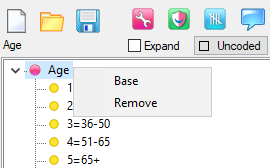
The Delete key also removes the current item.
You can rearrange by drag/drop or by the standard Ruby [Ctrl]-Arrow method.
Click on Frame to add a new codeframe. 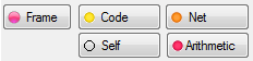
Code, Net, Arithmetic and Self add different types of code items.
Duplicate codes get added through drag/drop.
The Name, AKA and Label fields appear for codeframes in a hierarchic variable but not for a simple variable because they are the same as the fields for the variable itself.
Name becomes Code when codes are selected.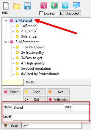
These are Hit-Enter-For-Next type fields. Make changes, press [Enter] and the next line is automatically selected with the cursor in the same position if possible - cycling around to the first line after the last.
This makes it easy to do quick repetitive edits.
A Base button and field appear at the bottom when a codeframe is selected.
You can type in the base expression here or select/build it in the Base form by clicking the Base button.
All codeframes can have a base - a code or pseudo-code or expression that provides the denominator for doing row and column percentages.
Either type directly into the field or click the Base button to build a base expression in the Select Base form.
Dragging into the codeframes field
Dragging variables or codes into the codeframes panel creates duplicate references.
Drag a variable and the duplicate is var(*), meaning copy all codes.
Drag codes and the reference is to those codes only.
Codes
Ordinary codes appear as a yellow dot.
Click Code to add a new one.
You can change the code and the label.
You can rearrange codes by dragging or with the [Ctrl] Arrow keys.
You can flag some codes as 'Exclude from sorting' (Brand10 has a white cross in the yellow dot)
This means that when a table of this variable is sorted, codes 1-9 will be in sorted order and code 10 will always be after all other codes no matter what its cell values.
When a variable in a table is sorted the order is:
sorted codes
codes excluded from sort
sorted arithmetic and nets
arithmetic and nets excluded from sort
Duplicates
Sometimes it is useful to mark one codeframe as a copy of another so that only the original need be changed at update time and all the copies are automatically kept in sync.
You achieve that by dragging a codeframe from the variable tree into the frame tree you are editing.
If you take the whole codeframe it is recorded as, for example, BPRF(*) meaning all codes, including new ones that are added at update time.
If you take just some of the codes it could be recorded as BPRF(1/6) - this is a static range and will not change at update time.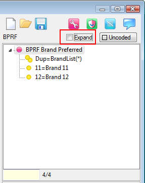
Duplicates appear as double yellow dots.
The Code field is meaningless and the Label field is the expression defining the duplicate: variable(code range).
You can shift codes as they are being duplicated by appending +/- numbers.
Gender(*) makes codes 1 and 2
Gender(*)+3 makes codes 4 and 5
Gender(*)-3 makes codes -2 and -1
You can mix duplicates and normal codes. You can take copies of codes from any number of variables and have multiple duplicate code line items.
The Expand switch in the top right allows you to see what the expanded version of the codeframe is after all the duplicate lines have been replaced.
If the codeframe for the duplicate had a code 10, and there was also an original code 10, the original one always has precedence.
This means that you can do some local relabelling of codes.
A check is made at job load time for circular Dup references. If you have Var_A as a duplicate of Var_B, and Var_B as a duplicate of Var_A, that's an impossible situation, and Ruby will issue a warning.
Arithmetic
Arithmetic items appear as red dots.
These are variously called:
Codeframe Arithmetic (because defining new codes based on existing codeframe items)
Raw Crosstab Arithmetic (because they define row/column arithmetic in raw crosstabs)
Codeframe arithmetic is the second level of calculation you can do on data. See Algebra.
The Code is the expression defining the arithmetic item. Clicking on the Arithmetic button opens the Arithmetic form for building expressions with drag and drop or by direct editing.
You can also exclude expressions from sorting.
Nets
Net items appear as orange dots and represent case level netting of responses.
These appear in the vartree after codes and before arithmetic.
Highlight the codes you want to net
Click Net
Label the new net as South (the net of SE and SW)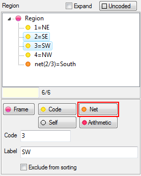
This creates a Net node similar to an Arithmetic node - you can edit the code scoping and the label.
You cannot change the 'net' text to any other function.
These are special nodes and netting is the only function presently available.
It gives the same result as the case function net_Region(2/3) but saves you having to create a function node on the specification form and is much faster.
It differs from the Arithmetic line #sum#(2/3) because sum includes repeated codes and net does not.
Unlike Arithmetic nodes that can be created on the fly (e.g. when defining a custom base or writing GenTab syntax), _net expressions can only be created in the Variable form, and are distinguished in syntax by a leading underscore.
Self-coding
Sometimes there is no information for a codeframe or the variable is quantitative and does not have a codeframe.
For crosstabulation, the variable can be flagged as self-coding.
Self-codes appear as white dots and have a different panel for editing the item's details.
The codeframe can be generated as a number of bands.
Ruby looks at the data file, identifies the largest and smallest values and divides it up into equal width bands.
Click the Expand switch to see how it will appear.
The codeframe can be generated in even steps.
Ruby looks at the data file, identifies the largest and smallest values and generates as many steps (code items) as are required to cover all the values.
Click the Expand switch to see how it will appear.
The codeframe can be a one-to-one mapping of all possible values.
Ruby sorts the data and makes every unique value its own code. Click the Expand switch to see how it will appear. This is useful for data such as postcodes.
Hierarchics
Defining missing information for hierarchic variables requires making sure you have the code range properly specified.
If the range is “*” it means the entire variable has no data for the filter expression.
Any other range must be compound having as many bits separated by ':' as there are levels.
You can type everything in but if you want to drag codes then first select the codeframe in the top right list.
Notice the second line has the range as “*” and the first has a compound range “*:8/10” meaning codes 8-10 of the second level have no data for weeks 1-10.
Arithmetic form
Clicking the Arithmetic button on the Variables form opens the Arithmetic form.
The display shows the current codeframe, which may already have some arithmetic expressions.
Double-clicking on a line it will replace the contents of the edit field.
To add something to the expression, highlight one or more lines (using [Ctrl] or [Shift] multiselect) and either drag it/them to the edit field or click the arrow button.
If a function is selected at this time it will also be entered.
You can also directly edit the expression. The final expression should begin with # but if omitted it will be inserted automatically when the form closes.
See the Algebras discussion for a full description of the syntax here.
In summary you can use the following operators:
= equal
!= not equal
> greater than
< less than
>= greater than or equal to
<= less than or equal to
+ add
- subtract
* multiply
/ divide
? modulus division
% percentage of
^ power of
& logical AND
| logical OR
! or ~ logical NOT
>> Lead
<< Lag
Operands can be any of the items in the display or any constant
Because the expression sum# is subordinate to a variable, the 1/2 in sum#(1/2) means codes 1 to 2.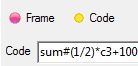
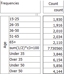
Code Lists
Code Lists are pieces of text that can stand in place of a list of codes. Some systems call these Macros or Substitutions.
Code lists are used in expressions like TMBA($BrandX) where the text $BrandX is replaced by the numbers at execution time.
Note the leading $ that indicates this is a code list.
Code lists are very useful for dynamic code groups or for a group which is used in many places because all instances can be changed simultaneously by editing the list definition.
The fields are arranged for quick keyboard entry of new lists:
[Alt]-N starts a new list (shortcut for New button 
The name field gets focus, type in list name
[Tab] goes to the list field, type in codes
Repeat the process starting with [Alt]-N
Click Delete 
Code lists are stored in job.ini.
Construct
Being able to construct new variables from existing data is an essential part of data processing and analysis.
Analysts can use the Tools|Banners & Nets Form for this purpose in most situations. The intention here is for analysts to have the capability to create the most common types of construction for themselves, without the need to call on DP.
The Construct Form contains more advanced features for single and multi-response constructions, date constructions and grid/cube or higher (hierarchic) constructions.
Once a variable is in the variable tree, and referenced in many reports or even other constructions, removing it can be difficult. It is worth a few moments to consider whether a construction is really necessary.
A construction is generally necessary for:
coded increments (price/brand, kilometres/vehicle, etc)
hierarchies
date variables
self-modifying variables which automatically recognises new codes
jobs with millions of cases, when on-the-fly as part of a specification may cost too much time
For all other requirements, try defining everything in a report specification first, and if for many reports, then append to the codeframe - only construct a new variable if absolutely necessary. For example, nets can be permanently added to a variable's codeframe via the Variables form or they can be added on the fly in the Report Specification Form. However, nets added via the Report Specification Form will be only available in the report in which they are created, and _net expressions from Edit Variables cost runtime. If the constructed variable is to be a permanent part of the job, in regular use for many tables and charts, then a constructed net is usually the best approach. If a net is only required for a few ad hoc reports, then an extra variable in the job is probably not worthwhile.
Most constructions are specified by defining a set of filters. Each filter defines the conditions under which its assigned code is written to the output file.
When the construction is executed, each case is tested against these conditions, and the code for each true condition is written to the target variable.
Three worked examples, using the supplied Demo job, are provided for a hands-on experience:
Example 1: Simple Crossbreak
Example 2: Complex Crossbreak
Example 3: Netting Codes
Using the new variables - report creation using each of the three newly constructed variables
Construct Variables Form
Both the Construct button on the Tasks group of the DP tab and the Advanced Constructions button on the Construct Variables group of the Tools tab open the Construct Variables form. This form is where you specify how to construct new variables from existing variables.
A lot can be done by drag and drop.
The lists and edit fields are set up to function much like text editors and there are generators that can do most of the work in straightforward cases.
Variable tree
The left panel is the familiar variable tree and its context menu for looking at a variable's data and ancestry.
You can drag things from here into the Filter and Increment edit fields, modifying them with the Case Data Function drop down if desired.
Double-click a variable to load it, or drag it to the far right panel.
Dragging codeframes or codes into the middle panel generates the next available code.
Lines
The middle panel defines the set of codes and increments, one line for each.
Click New Line or press [Alt]-N to add a new one.
Press the [Delete] key to remove the current line.
Clicking on a line shows its details in the Code/Filter/Increment fields ready for editing.
The Code, Filter and Increment fields are Hit-Enter-For-Next type fields.
Make changes, hit [Enter] and the next line is automatically selected with the cursor in the same position if possible - cycling around to the first line after the last.
This makes it easy to do quick repetitive edits for which you might otherwise turn to a general text editor.
You can construct the same code multiple times.
The first two lines define code 1 as both Age(1) and Occupation(3).
Frames - Levels
The right panel shows the construction's codeframe.
Click Frame to add a new codeframe (or level if hierarchic), or click Code to add a new code.
The [Delete] key deletes the current one.
Click Replace to bulk-replace text in code labels
If there is only one level this is a simple variable - the codeframe and variable have the same name (ensured when saving) and the labelling is simple.
When there are more levels it is a hierarchic variable and the codeframes are labelled as Variable.Frame.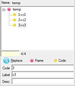
The Code and Label fields are Hit-Enter-For-Next types that cycle through all the items in the list, making it easy to do quick repetitive edits.
Match
When the script is run the codeframes are forced to match the construction lines.
You may want to do this manually at various times as you are building up the script.
The left Match button 
The right Match button 
This means you can work either way - set up the codeframes and labels before deciding on the filters, or set up the filters first.
The filters and the labels cannot be specified in parallel.
This is because there is not a one-to-one correspondence, because either the same code is defined multiple times, or because the constructed variable is hierarchic.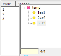
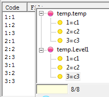
On the left the codes 1, 2 and 3 match the labels c1, c2 and c3, but on the right there are 6 code labels, but nine filter expressions.
Generator, Dates and Grid - Always Generate
The Line, Date or Grid generators can auto generate filter lines and code labels.
The Always Generate switch 
If checked, and the generator has something in it, it will be run again and any existing lines and codes completely replaced by the generation.
This is a good idea for a straightforward construction that needs to keep pace with new data, adding new codes and construction lines as necessary.
It is a bad idea for a construction that requires manual intervention.
If the generated output was used as a starting point for further customisation, then Always Generate should be OFF - otherwise the customisations will be lost.
New, Open, Save
New: starts off a new construction from scratch, naming it 'temp'.
Open: displays a File Open form. When the variable is selected, the .MET file opens and the form displays any construction information in the variable.
Save: saves the variable's metadata (codeframe and construction data) to a .MET file, with the provided name.
NB: Saving the .MET file does not create the associated .CD file (the data file). The .CD file is created when the construction is Run.
In some situations you may just require the .MET file without the .CD file - e.g. when creating a reference codelist file for use in scripted constructions. If so, never use the Construct form - use the Edit Variable form instead.
Run - Output switches
On clicking Run the .MET is saved and the construction is run.
Codes & Increments
If both Codes and Increments are ON, the .CD file will contain data like 3*1.5 where 3 is the code and 1.5 the increment.
The default coded increment 1 is not written - for example 3*1 is written as just 3 to save space.
Increments of zero are written out as 3*0.
All uncoded increments are written.
If Output Increments is OFF, then just the code is written, even if increment expressions are present.
If Output Codes is OFF an uncoded data file is generated.
The .MET file will not have a codeframe, the frames panel will be empty and all code column entries will have * instead of a number.
The .CD file will just have the increments without the * separator.
NB: The asterisk is used in more than one sense: as a missing indicator for codes, and as an increment operator.
To the extent that 3*4 is the same as 3;3;3;3, the increment operator is the same as 'multiply'.
Add to Tree
If the variable was already in the variable tree it will be refreshed.
If Add to Tree is checked and the variable is not yet in the tree it will be added to the bottom.
You can do some rearranging here - drag the variable to a folder - but full editing of the tree is only available in the Edit Variable Tree form.
Tidy Hierarchic Data
If you are constructing a hierarchic variable, you may end up with data that is not neatly organised.
For instance, a1b2a2b3a1b4 is more economically expressed as a1b2;4a2b3 - the two disassociated a1 branches have been merged.
This switch organises each case data into the neatest possible tree structure before writing it out. But note that this may affect crosstab outputs, since in the untidy form, a1 will be counted twice.
Top Up Only
Normally every case is constructed to ensure always consistent with its ancestors. However, some constructions can take a long time, since all filters must be evaluated for every case. With this switch ON only new cases are constructed. A short .CD file will be extended to full length but a full one will not be changed.
Net Responses.
Constructions can produce output with duplicate codes, especially when the source is hierarchic.
1;1;2;3;3;2;1;2;2
With the Net Responses switch ON the duplicates are removed
1;2;3
Dragging Codes
If you drag codes into the middle panel each one generates another construction line (using the next available code) and a matching label in the codeframe.
Dragging Variables
If you drag variables into the middle panel you still only get one construction line (not one per code, as you might expect) using the next available code but the label generated in the codeframe is now the description of the variable.
This behaviour makes it easy to deal with dichotomised variables.
For example, a logically multi-response variable in SPSS will import as a separate variable for each code, and these variable descriptions will become the code label when assembling to a single multi-response variable by dragging each dichotomous variable in turn.
Dragging a variable into the codeframes panel on the right is the same as double-clicking it. It is a signal you want to load the variable.
There is a prompt to confirm.
Line Construction Generator
The Generator button 
This form specifies the rules for generating a construction script.
Most of the fields have substitution features that are fairly simple in principle, and can be very powerful in practice.
Usually you would do Date and Grid constructions using the Date and Grid generators but on occasions you might need the extra flexibility available here.
For example, if the source variables are consistently named it is possible to specify a 3D grid here much more quickly than by dropping all the variables on cells in the Grid Generator.
The first few examples demonstrate the more straightforward techniques available. The later ones are more complex.
The left panel is the familiar variable tree.
There is a context menu for looking at a variable's data and ancestry and a Collapse All item to tidy up the tree.
You can drag things from here into the Levels panel.
You can drag to the Filter and Increment fields, modifying them with the Case Algebra Function drop down if desired.
The top right panel shows the Levels (codeframes) that will be generated and the bottom panel shows a template of the construction lines.
The three switches at bottom left control how the generation is performed.
You can very quickly build recode scripts, separate hierarchic variables, loop to create hierarchic variables, unloop to flatten hierarchic variables, merge variables, aggregate date variables, etc.
There are a few concepts to become familiar with but the system has been designed to make obvious things easy, best demonstrated with a few examples. 'From a clean start' means with all fields empty in the form.
A quick way to get this is to click the New button
Example 1 Just generate some codes: Label=$
From a clean start click the New Level button
Run
On the left is the Generator form and on the right the result of the generation in the Construct form.
This generates every code in the range 1 to 10 and labels them as 'Code n' where n is the code number.
Labels- $
The $ character in this context means substitute the code number. 1/10 is the default range.
It can be discontinuous like 1/5,8/14,20 or 1/5;8/14;20 if you are accustomed to using ';' rather than ',' (actually, any delimiter will work here).
'Code $' is the default text and can be anything with $ any number of times.
Each $ will be replaced with the code number so $$ would produce 22, 33 etc.
You can't have a literal $ character, though.
Example 2 Recodes
From a clean start drop a simple variable on the Levels box
Run
The default entries generate a construction that makes an exact copy of the original codeframe.
Code ranges
There is now a Source and the Range is the familiar * meaning 'all defined codes'.
This could be changed to any legal code expression like:
1;3/8;11 conventional integer code range
4.2;7.5/11.5;21 decimal code ranges
1;3/40;~9/10;15 everything after tilde excluded
* asterisk means all defined codes
*;~5 everything but code 5
N-13 last 13 codes (see example 4)
Labels - $var($)
The Label field shows two extra substitution devices.
$Region() means to copy the code label from the variable Region, and what is inside the brackets determines which code labels to copy.
The $ in the bracket means the code number. You can also do some algebra here.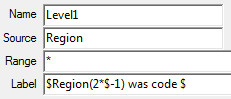
This shows all three different uses of $ substitution in labels.
The $Region identifies a codeframe from which to get labels.
The (2*$-1) substitutes each code for $ in turn and evaluates the expression.
The final $ outside the bracket, not prefixed to a name, is replaced by the number as text. You cannot do algebra on a $ outside parentheses.
The algebra in the brackets allows further brackets to any depth and the operators + - * / ^(power). Where the evaluation produces a code not in the frame you get the var(code) text.
At code 2, 2*2-1=3 so you get the label for code 3 (SW).
At code 3, 2*3-1=5 and Region doesn't have a code 5 so you get the text Region(5).
Filter - $a, $@a, $(a+1)
This introduces the simple substitution device available in filters and formulas.
$a means use the code from level A. (For a flat variable such as Region, there is only one level, being the codeframe itself).
Even without algebra interesting things are possible if you remember that $a is replaced anywhere, not necessarily in brackets.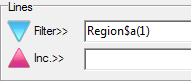
With four variables named Region1, Region2, Region3 and Region4 the $a can represent part of the variable name.
If the four variables are instead named RegionA, RegionB, RegionC and RegionD then you can use the alpha form of the substitution $@a to represent the name part.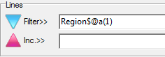
This will not make sense inside brackets, of course.
The 'a' bit can be any expression in brackets, so you can shift codes as for example Region($(a+1)).
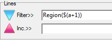
Once again, the algebra in the brackets allows further brackets to any depth and the operators + - * / ^(power).
Example 3 Uncoded
If the Uncoded switch is ON, then the Generator produces filters where the codes are missing and there is no codeframe.
You would do this to create an uncoded file and would additionally need to have some formulation in the Increment field to supply an output.
Example 4 Last few codes: N-13
The idea here is to construct a new variable that is the last N codes of another.
A typical example is the last 13 weeks so a chart of previous quarter updates automatically.
From a clean start drop Week in the levels field
Change the range to N-13
Turn on Sequential Codes
Run
The result is a new codeframe always numbered from 1 that recodes the last N codes from the source.
The signal in the range expression is N- followed by a number.
Example 5 Extract hierarchic levels
From a clean start drop the hierarchic level BratRats.Brand on the Levels box
Run
This extracts all the brand level responses from the hierarchic variable into a flat variable.
In the Construct form:
Save as Brand
Run
To check the construction, right click on Brand and select Data, then right click in the Brand column and select Ancestors.
NB: This breaks the connection with the other parts of the hierarchic variable. The output comprises the brand codes 1 and 2 only.
Example 6 Unloop
To create a single flat variable that retains all the connections with the other levels of a hierarchic variable, you can use the Unloop switch.
Drop each BratRats level in turn into the Levels box
Check Unloop
Run
The output is
The convoluted filters covers every possible combination of brand, attribute and rating, and the codeframe has been assembled by concatenating the relevant codes.
It is conventional to name it by simply appending an 'F' to the original name.
Save as BratRatsF
Run
Inspect BratRatsF and its ancestor.
Example 7 Aggregating codes: Range=$()
From a clean start drop the Day variable on the Levels box
change the Range to $(5*#-4)
change the Filter to Day($a/$(a+4))
Run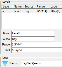
This generation will make a construction for a Week variable although note that it is not a Ruby MJD date variable.
This is just a conversion of one numeric variable into another that nets codes in a formulaic way.
The first five days constitute week1, the next five week2 etc.
Range - $(#)
This introduces algebra in the range field, an expression inside $(), and the special character #.
This just means sequential numbers - start at 1 and go up by one until generating a code that does not exist in the Source.
Think of it as 5n-4.
The first code will be 5*1-4=1, the next 5*2-4=6, the next 5*3-4=11 etc.
When # reaches a code that Day does not have, the process stops.
# is the only substitution character possible here but you can use brackets to any depth and the operators + - * / ^(power).
Filter - $a/$(a+4)
The expression uses both forms of level substitution.
$a means the code at level A and $(a+4) is that number plus four.
Sequential Codes
The above does not produce sequential code numbers because the code number is always the code at that level - effectively always $a - and the Range expression produces the sequence 1,6,11,16...
You can get sequential code numbers by setting that switch back on the Generate form.
Labels - #
One final substitution possible in labels is the # character itself.
Remember that # is always just sequential numbers from 1.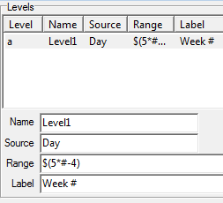
Example 9 Grid question: Filter $a $b, Label=?()
Logically hierarchic questionnaire data is often imported as sets of flat variables.
These should usually be combined into a single hierarchic variable.
BIM and BEQ in Setting up the Demo Job are examples of these.
The Grid Generator provides a more visual alternative.
Filter patterns
If there is a pattern in the filters, then the entire grid can be assembled one line per level.
For instance, the BIM filters end up like
1:1 = BIM1(1)
1:2 = BIM1(2)
1:3 = BIM1(3)
2:1 = BIM2(1)
2:2 = BIM2(2)
2:3 = BIM2(3)
This is of the General Form a:b = BIMa(b)
The first level code ends up being part of the variable name and the second level code is the code in brackets.
Therefore, the filter is simply BIM$a($b).
From a clean start click the New Level button
Change the range to 1/3
Drop BIM1 into the Levels box
Change the filter to BIM$a($b)
Run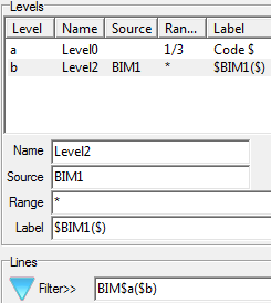
The second level codeframe is supplied by BIM1.
The first level codeframe needs to be made from the descriptions of BIM1, BIM2 and BIM3.
Padding Zeros
1:1 = BIM01(1)
1:2 = BIM01(2)
1:3 = BIM01(3)
2:1 = BIM02(1)
2:2 = BIM02(2)
2:3 = BIM02(3)
If the variable names have the numbers padded with zeros you can indicate that with multiple $ characters.
For example
var$$a_$$$b
produces the following pattern:
var01_001
var01_002
var01_003
var02_001
var02_002
var02_003
...etc
Labels - ?(var$), ?(var$@)
Return to the Line Generator
Click on the first level
Change Label to ?(BIM$)
Change Level names to Brand and Statement
Run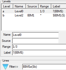
The ?() syntax means 'Description of variable in brackets'.
Inside the bracket is BIM$ that will be BIM1, BIM2 and BIM3 in turn.
The labels may need to be cleaned up a bit, just as from the special Date Generator.
You can also have letters generated by using $@ instead of $. ?(BIM$@) generates BIMa, BIMb, BIMc.
3D Grid
You can also generate the 3D BEQ grid.
The BEQn variables are each for a specific Brand/Statement combination, all with the same codeframe - the 1-10 Rating scale.
Any of these can supply the codeframe for the third dimension, but getting the other two can require some creativity.
The second dimension has to be the seven statements so the codeframe could come from the descriptions of the first seven BEQn variables using the ?() syntax, or you could create a dummy variable to hold the codeframe as described in the Grid Generator 3D example.
The first dimension requires three codes for the Brands.
In this example it is assumed that you have created a dummy variable BrandList with a codeframe BrandX, BrandY, BrandZ.
From a clean start drop BrandList in the Levels box for the first dimension
Set Name to Brand
Click New Level for the second dimension
Set Name to Statement
Change the Range to 1/7
Change the Label to ?(BEQ$)
Drop BEQ1 in the Levels box for the third dimension
Make the Name Rating
Change the Filter to BEQ$(7*a+b-7)($c)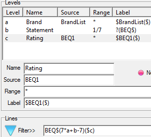
The Filter expression shows how sophisticated you can get with the algebras.
The 'a' and 'b' values combine to make the result 1,2,3 up to 21 as 'b' goes from 1-7 inside 'a' going from 1-3.
Syntax Summary
In the following an expression is indicated like (…x…) where x is a character that may be used as an algebraic variable.
Expressions that can be evaluated always appear in brackets, usually $() except for $var().
Range $(…#…) or @(3m 1jan2004) or N-13
Normal code ranges like 1;3/8;11, *, *~5.
N- followed by a number for last n codes.
$() enclosing a # expression where # is 1,2,3… until resulting code is not in source.
@() containing a date cycle.
Label text $var(…$…) # text $ text @(ddmmyy) ?(var$@)
Any other text is copied.
$ immediately followed by an alpha is expected to be a $var() formulation that returns labels in var for the code that results from the (…$…) expression.
$ not followed by alphabetic char is replaced by code.
# is the ordinal line number.
?() returns the description of the variable in brackets - handy when variables have a numeric component in the name and can be built using $. ?(var$) replaces $ with codes, ?(var$@) replaces $@ with letters from codes up to 26.
Filter and Increment text$a $b $c $(…abc…) $@
Any other text is copied.
$a is code at level A, $b code at level B etc, for as many levels as you have (it does not stop at C).
$() can enclose an expression using any and all of the level characters.
$@ followed by levels or bracket expressions returns lowercase letter from 1=a to 26=z.
Multiple $ characters mean pad with zero. e.g. var$$a_$$$b for var01_001
Date Construction Generator
The Dates button 
There are some other ways to generate date constructions in the Line Generator but the simplest is to use the dedicated Date Generator.
There are three common circumstances covered by this form:
Convert a numeric variable like WeekNumber with a simple codeframe like 1, 2, 3, 4… into a proper date variable
Convert a date variable at one cycle (e.g. daily) to another date variable at a different cycle (e.g. monthly)
Convert a text variable whose codeframe contains date strings into a usable date variable
Convert Numeric Date
Here the source variable WeekNum (not in the Demo job) is a week number categorical variable with no calendar gaps.
To construct a week date variable, drag this into the Source field, set the Date Cycle to 1 Week, and set the Start to indicate the first day of the week.
Here 1Jan2000 is a Saturday, but any Saturday will produce the same result.
The Format field determines how the date labels will be generated and takes strings similar to those used in the Control Panel tool Regional and Language Options|Customise|Date.
For example, mm means numeric month number (two digits), mmm means abbreviated month text (three characters) and mmmm means full month names.
Ruby additionally allows Q, QQ and QQQ to stand for quarter labels like Q1, Qtr1 and Quarter 1.
Characters other than d, m, q and y (upper or lower case) are copied verbatim. The default is dmmmyyyy.
Clicking Run produces the following back in the Construct form:
The code labels for the construction are proper dates, and the construction lines simply map the numeric codes from the source variable onto those.
Note the requirement for a straight numeric conversion is that the source must have no calendar gaps. To demonstrate using DayNum in the Demo job: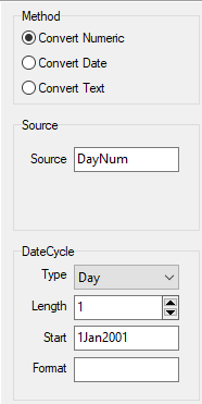
DayNum skips weekends, so there is no definition for 6Jan01 and 7Jan01, but these dates are spuriously generated.
See Gaps in Dates for a workaround. The other date conversion methods are generally preferred, if you have appropriate source.
Gaps in dates
For Convert Numeric, If there is a gap in the date record - for example no data for February - you can achieve that by deleting the later codes and running the generation again.
Note how the gap has been indicated by deleting most of the later codes and making the last one show the first date after the gap.
This gives the generator a reference to start from.
Clicking the Dates button and simply generating again gives the following:
Note how the dates are now refilled after the reference 4Mar2000.
This is actually quite different from the other generators (including the other date generators).
The codeframe is NOT cleared by the generation process, only added to and only just enough to match the size of the Source codeframe.
If you want all labels regenerated, then delete them first.
This approach also makes updating these straightforward.
At subsequent imports, the source variable will likely have new date codes.
If you have the Date Generator set to Always Generate, then when you update this construction it will first run the Generator (thereby extending the date codeframe) before running the construction.
Convert Date Example
This example shows constructing a Quarter variable from a Month date variable.
Select Convert Date method, drag Month into the Source and set the Date Cycle for 3 Months starting at the first month.
The format is set to qqq yyyy to take advantage of the special Quarter labelling.
Clicking Generate gives the following.
You can generate a Month variable from a Week variable but it will just be some four-week collections and some five-week collections.
To get an accurate Month variable you need to start with Day.
The codeframe is always cleared and regenerated from scratch.
See the Quarter variable in the Demo job, which was constructed using this method.
Convert Text
Sometimes date information is mixed in a text string within the data like Sun Feb 12 04:44:19 CST 2006.
This will be collected as Text data into a variable whose codeframe will be each unique text string.
This converter generates an MJD date variable from that codeframe.
This is a special construction because it does not involve recoding or combining codes.
There is only one construction line with a special filter expression to invoke the special processing.
The Date Constructions generator form identifies the source variable and indicates how to find the date information in the label text with a format string.
This uses the characters 'd', 'm', 'y' to mean Day, Month, Year and 'w' to mean a padding word.
In the example dmyw means the first word is day, the second is month, the third is year, followed by a word of no interest, being the hour:minute:second:thousanths.
The codeframe is generated as part of the construction run itself.
The codeframe date format is also specified.
One other format character '@' means a complete date string.
e.g. The string Begin Sun 12Feb06 04:44:19 would have a format string ww@ indicating the complete date appears as the third word.
As long as the date string is not ambiguous Ruby will tolerate a wide set of styles.
e.g. 2011-10-18 is recognised.
Back in the Construct form, note the special filter expression (the code does not matter).
The initial @ means this is a special date construction.
If the character after the @ is a letter it must be a variable name with the translation format inside brackets.
Codeframe from Construction, not Generate
Clicking Generate creates only the single construction line, which you could just as easily have typed in.
The codeframe is generated as part of the construction run itself.
This is because code information is contained in the data, not the construction lines, so the codeframe cannot be known before the construction is run.
Special 3-variable Date Construction
There is one other special construction for generating a proper date variable from three numeric ones that hold the Day, Month and Year.
This method has no GUI yet, but is simple to create.
You make one construction line and type in the filter like @3s3day,s3mon,s3year.
The critical characters are the initial @3 highlighted in red.
The @ means a special date construction and the 3 means the 3-date method.
These must be immediately followed by the three numeric variables separated by commas in Day, Month, Year order.
Again, the codeframe only appears after Running the construction.
Inspecting the data for Day and adding Ancestors makes the relationship clear.
Note that the year variable has small numbers.
Ruby assumes numbers less than 100 are in the window around 2000 from 1950 to 2049.
Grid Construction Generator
Clicking the Grid button on the Construct form opens the generator for constructing two or three level hierarchies.
You generally find these on questionnaires as one or more grids and they are usually stored in many flat variables.
Sometimes it is one variable for each row (or column) and sometimes it is one variable for each cell.
2D: Each Row (or Column) is one Variable
The Brand Image variable from the document Setting Up the Demo Job.pdf is an example of this.
The variables are usually in a set all with identical codeframes.
In the Grid Generator you:
Use one of the variables to supply the codeframe for one edge of the grid (BIM1 in Side Codeframe)
Set the size of the other edge with the thumbwheel (Top = 3)
Drop each block of variables into the column headers
Multiselect-drop is convenient if the variables are in the right order. They will fill out the column or row headers from the point where you drop them in order until either the columns or variables run out.
Give a proper name to the levels
Generate
You could equally build the grid in the other orientation - supply a codeframe for the top and drop variables on the side.
Back in the Construct form you can see how the filters are generated from the variable names in the column headers and the code in the rows.
The codeframe for the top level has been generated from the descriptions of the variables and usually needs to be cleaned up a bit.
From here you:
Clean up the codeframe that came from descriptions
If there are only a few you can do it manually using the hit-enter-for-next feature of the Label field.
If there are many you can use the Replace form.
Give the new variable a description
Save and Run
3D: Each Cell is one Variable
The Brand Equity example in the document Setting Up the Demo Job.pdf is an example of this.
Usually they are clearly three dimensional - for each brand, against each statement there is a rating - but in highly atomised field systems that can't hold multi-responses you can end up with a 2D grid question where each cell has been stored as a separate variable.
The variables are usually in organised blocks.
They usually all have the same codeframe but it is for the third dimension and can't be used to provide the labels for one edge of the grid.
Sometimes you can find another variable in the job that can serve for this (as in the BEQ example below, which uses ABA) but sometimes you have to manufacture a dummy variable.
In the Edit Variables form you:
Start a new variable
Add as many Codes as required
Edit the labels
Save
This creates a .MET file and there will never be a .CD file.
All the variable is doing is holding a codeframe you can use in the Grid Generator to provide the labels for one edge of the grid.
The process begins exactly as for the 2D case except the codeframe for one edge does not come from one of the source variables.
It might be from somewhere else in the job or it might be a dummy one created in the Edit Variables form, as above.
Use a dummy or other variable (here ABA) to supply the codeframe for one edge of the grid (here, the top)
Set the size of the other edge with the thumbwheel (here, to 7, the number of statements)
Drop the first block of variables (the seven statements for BrandX) onto the labels of the other edge
It does not matter which block of variables were used in the last step - all you are doing is supplying code labels from the descriptions of the variables.
The filters will be made from the variables dropped in the cells in the next stage.
Any of the rating variables can be used to supply the codeframe for the third dimension.
For the body of the table, if the variables are in the correct order you can drop them as a block - but take note of the “Fill Body Cells” switch at the bottom left of the form.
The cells could be filled row by row (Horizontal) or column by column (Vertical). If they're not in a tidy order you can drop them individually into cells.
Drop any one of the variables into Level 3 Codeframe
Drop the block of variables in the first cell
Give the levels proper names
Run
If you make a mistake dropping the variables in cells, then simply drop the correct variable on top of the mistaken one to replace it.
To clear a cell, use the right-mouse menu item Remove.
Back in the Construct form, each cell variable creates one filter for each code in the third dimension.
Again, the code labels that came from the original descriptions will need to be cleaned up.
A neat way to do this is click on one, highlight the text to be removed, copy it, then open the Replace form and paste it in - click Ok to replace with empty text.
Clean up the codeframe
Give the new variable a description
Save and Run
Example 1: Simple Crossbreak
Existing codes can be dropped into the middle panel on the Construction form.
Click new
Open the Age variable in the tree on the left
Multi-select codes 1 to 5 using [Ctrl] or [Shift] click
Drag these into the middle
Note that each dropped code generates two things: a construction line in the middle list with a code and filter expression, and code with label in the codeframe tree on the right.
Open the Gender variable and do the same for codes 1-2 of Gender
Click Save
Click Run
A message should appear saying the run was successful, and Crossbreak1 is appended to the variable tree.
The new variable can be used immediately in tables and charts.
This is a quick way of assembling a crossbreak or similar recoding.
The behaviour is fairly obvious - dropping a code in the middle creates a new construction line for the next available code, sets the filter to the just dropped variable(code) and copies its label.
At any time, you can change the codes, labels and expressions, or enter a description of the new variable in the VarDesc field at the bottom right.
Changes to labels or descriptions are preserved simply by clicking the Save button.
Changes to codes or filter expressions - anything that would change the constructed data - necessitates running the construction again.
Dragging Variables
If you drag just the variable name, then it drops as the variable filtered to code 1, with the variable description being used to supply the code label.
This technique makes it easy to reassemble dichotomised variables - typically where a conceptually discrete multi-response variable has been split up into many separate variables, one for each code, as 1=yes, 0 or 2=no. This can happen when importing several common file formats, such as SPSS *.sav or *.sps/asc.
Example 2: Complex Crossbreak
This example builds a crossbreak with compound and netted filters for things like females under 35.
Start a new construction
Click New Line 
Open Gender in the Variable Tree and drag Female to the Filter field
Open Age, highlight codes 1 and 2 and drag to the Filter field or click the Filter button
This filter means Females under 35.
Click New Line
Set the second filter to be Gender(1)&Age(1/2) meaning Males under 35
Click New Line
Find Married in the Variable Tree and drag No into the Filter
Find Occupation in the Variable Tree and drag codes 1-4 into the Filter
This has made three new definitions: Females under 35, Males under 35 and Employed singles.
To give them labels
Click the 
Click on the first code, 'Code 1', in the codeframe on the right
Its label and code appear in the edit fields at the bottom.
Change the label to Females under 35
Press [Enter]
Focus jumps to the next code, its label appears ready for editing and the cursor stays where it was in the Label field.
Change the second label to Males under 35
Press [Enter]
Change the third label to Employed singles
Click Run 
Save
The new variable has been added to the bottom of the tree.
To inspect the data and check the construction is as intended:
Find Crossbreak2 at the bottom of the tree
Select Data from the right-mouse menu
This opens the Variable Data form where you can inspect data.
Right-click in the Crossbreak2 column and select Ancestors
This adds every other variable that was used in the construction.
It is easy to confirm that the construction is correct by referring the codes for GEN, Age, Married and Occupation to the constructed code for Crossbreak2.
Click on a column header to see the variable's codeframe
Click on any code in any column to see the decode in the bottom panel
Close the Variable Data form
Example 3 Netting codes
In this example it is assumed that the ten brands in the Brand Preferred variable can be grouped into three major brands.
To net the ten variant brands down to the three parents:
Click new
Press [Alt]-N or click the New Line button
Find Brand Preferred under the Behaviour folder in the variable tree and show its codes by clicking the + if they are collapsed
Select the first three codes and drag them to the Filter field or click the Filter button
This sets up the first construction line and the next few steps show how to quickly add and edit similar ones.
The controls are organised for quick keyboard entry. [Alt]-N starts a new line and [Tab] cycles through the code and filter fields.
Subsequent lines are copies of the previous one with the code number increased, which is often convenient.
Press [Alt]-N to make the next line
The code is incremented to 2.
The code edit has focus, code 2 is what you want
[Tab] to the next field
The Filter field gets focus, edit the expression to be BPRF(4/7)
Press [Alt]-N to make the next line
The code edit has focus, code 3 is what you want, [Tab] to the next field
The Filter field gets focus, edit the expression to be BPRF(8/10)
That creates the filters, but there are no matching code labels yet.
Click the Match>> button
Editing codes and filters is very convenient because the Code, Filter and Increment fields are Hit-Enter-For-Next type fields.
Click on the first code on the right and edit the label to be Major 1
Press [Enter]
Note the highlight jumps to the next code, its label is in the field ready for editing and the cursor stays where it was.
Change the second label to Major 2
Press [Enter]
Change the third label to Major 3
Save
Click Run
The Hit-Enter-For-Next fields avoids switching from mouse to keyboard for repetitive edits. Direction is forwards with cycle back to top on the last item.
Using the new variables
The newly constructed variables from Examples 1, 2 and 3 are immediately ready for use in tables and charts.
The use of the three constructed variables in reports is detailed in this section.
Crossbreak1: (created in Example 1: Simple Crossbreak )
Close the Construct form
Start a new table
Drag Crossbreak1 to Top
Drag Region to Side
Click Run
Crossbreak2: (created in Example 2: Complex Crossbreak )
Start a new table
Drag Crossbreak2 to the Top
Drag Region to the Side
Click Run
Netted codes: (Nets created in Example 3: Netting Codes )
Start a new table
Drag Week to the Top
Drag Majors and its ancestor BPRF to the Side
Click Run
The Major 1 row should be the sum of the first three brand rows (because BPRF is single response) and this is indeed the case.
Constructions - Concept Explanations
New variables can be constructed from any others using a variety of recoding and code mapping techniques.
An ordinary construction in Ruby is a set of conditions which define under what circumstances a particular code and optional increment will be generated.
e.g. 1 = Age(3/5) means a code 1 for the new variable will be generated for any case which has a code 3, 4 or 5 in Age.
The filter expressions can be simple or very complex.
The document Setting up the Demo Job.pdf covers most of the construction techniques.
Filters
Netting things together is done by OR-ing them.
1 = s25(1/3)|s27(2;5/7)
This produces a code 1 if s25 has a 1 to 3 or if s27 has a 2, 5, 6, or 7.
Note how the range separator is a semi-colon and not the more common comma.
This is to avoid problems with the international notations where a comma is used for a decimal point.
More complicated conditions can use other comparators
1 = (sum_spend()>25)&visits(1/4)
With judicious naming of variables, these expressions can be very readable.
This constructs a 1 if visits has a 1, 2 3 or 4 and sum of spend (or just the value if single response) is greater than 25.
There are two interchangeable boolean negation operators, ! and ~.
1=Age(1/3)&!ABA(1)
1=Age(1/3)&~BYREG(1)
While the meaning is identical - sometimes ~ is more readable than !
Increments
Ruby data items can be incremented.
e.g. 3*2.5 might mean the respondent spent $2.50 on brand 3, or it might mean there was an order of 2.5 metres of cloth type 3 etc.
The 3 is a category code and the 2.5 is the increment.
At cross tabulation time, the 3 indexes a row or column, and the 2.5 is the value added to (thereby incrementing) the indexed cell.
All codes have a default increment of 1.
Construction scripts can also generate increments. The expression syntax is identical to the filter syntax.
However, the result of the calculation is not just true/false but an actual value.
e.g. If the first four cases of the Age variable have responses 1, 2, 3 and 4, then Age(3/5) will return 'false', 'false', 'true', 'true' as a filter and '0', '0', '3' and '4' as an increment.
Note how the range expressions work in increments - if the response is not in the range then zero is returned.
Default Case Functions
The example with sum_spend() shows the use of functions.
Ruby has many case functions that can be applied to a variable, such as sum_, net_, avg_, etc.
They are always three characters followed by an underscore.
All variables have an implied function depending on context.
This is why Age() gives true/false in a filter and the actual code value if an increment.
In filters the default function is net_.
When Age(3/5) is in a filter expression it really means net_Age(3/5) - meaning return true (actually, the value 1) if there is any Age code between 3 and 5.
In increments the default function is sum_.
When Age(3/5) is in an increment expression it really means sum_Age(3/5), which evaluates to the sum of any Age codes between 3 and 5.
Since each case will only have one response for Age, the sum is the actual code value.
You can use net_ in increments and sum_ in filters.
You can use any functions anywhere - but just remember that the default filter function is net_ and the default increment function is sum_.
The default increment function is also assumed in weighting expressions.
Any Boolean expression or sub-expression evaluates to 1 for true, and 0 for false.
Some standard variables
If not supplied by the source data, a Count variable and a Case variable should be constructed.
See Setting up the Demo Job.pdf for details on this.
Count
Count crosstabbed against any variable shows the distribution across the codes.
This is simply a stream of 1s and can be constructed in one line.
1=Day()|1
There may be missing cases, hence the |1, so that the filter Day()|1 will return true if Day has any value, or 1 (true) if the response is empty.
You can use any variable instead of Day. It is best to use a simple single response.
Case
Some field systems provide a variable with a unique case number.
If not, you can construct one in a single line that numbers the cases in order using the cum_ function as an increment.
*=1 cum_Count()
In this line the code is missing (*) because Codes is unchecked, the filter is 1 (always true) and the increment is cum_Count().
This function is unique in that it operates across cases. Count is a stream of 1s and this will be the cumulative sum of those 1s.
The output needs to be uncoded otherwise it would be 1*1, 1*2, 1*3 etc. With Codes OFF the output comprises increments only, generating just 1, 2, 3 etc.
To give Case a permanent codeframe, define it as self-coding in the Edit Variable form.
Usually a Case variable is left uncoded. If you use Case as a table axis it will self-code on the fly.
Some neat tricks
Other Mention from First and All
A questionnaire might have What brands are you aware of? and the first is stored in a separate variable.
Given the source variables Q21 and Q22, to construct a new variable Other Mentions that is everything but the first mention
Open the Line Generator form
Drop either Q21 or Q22 in the Levels panel to supply the labels and code range
Edit the filter to Q21($a)&~Q22($a)
This delivers codes that are in Q21 and not in Q22.
Making Increments
Increment expressions can use the same syntax notation as filters.
A simple example is constructing an elementary loyalty measure from a usage variable.
If brnd1 to brnd3 are variables saying how many of each brand were bought, then loyalty can be inferred from a variable which associates each brand with the number bought.
These each say If the respondent bought at least one of this brand then output the brand code with the number bought as increment.
1=sum_brnd1()>0 brnd1()
2=sum_brnd2()>0 brnd2()
3=sum_brnd3()>0 brnd3()
A crosstab of this new variable will show the actual number of items bought for each brand (as opposed to the number of respondents who bought a given number of brand items).
Weights
Use the Weights command on the Tasks group of the DP tab to open the Weights form.
The general idea of weighting is to look at how many respondents you got as opposed to how many you wanted, and to then calculate a weighting factor for each case accordingly.
For example, on a sample of 50 per week, you may want to always have 25 males and 25 females.
In week#1, you actually have 30 males and 20 females. So the weighting factor for males is 25/30=0.833333 and for females, 25/20=1.25.
On the left is the familiar variable tree.
The panel on the right is the definition of weight variable - the target percentages for various codes - and there are a few controls on the bottom for the type of weight to generate.
Cell or Rim: Weights are determined by target percentages in cells or on the 'rim'. Cell targets are the product of combinations of code percentages. Rim targets are the code percentages themselves.
Rim weighting is an iterative algorithm that generally converges. You can control the convergence limit and the maximum iterations before leaving a non-converging attempt.
Respondents or Population: With Weight To Population checked the figures are scaled up to proportions of that figure.
Within Periods or Total Sample: If a Period variable is supplied the weights are caculated independently within each period.
Write Report: When a weight construction is run Ruby can create a companion reports file *.WRP, same name as the variable, in the CaseData directory.
This shows marginal and cell information plus standard weight efficiency stats.
You can turn this off for the run in this form with the Write Report switch.
Rim convergence failures are additionally written to a common Weight.log file in the job directory.
Here is an example Weight Report:
Weight Report: WghtAgeGenRegRim
Marginals .........................
Input Input Target Target
Frequency Percent Frequency Percent
GEN --------- --------- --------- ---------
Male 4985 49.85 4000 40.00
Female 5015 50.15 6000 60.00
RIM Summary .......................
Converged on iteration 4 with SSF=0.00000239 vs limit 0.00010000
Rim Output Output
Weight Frequency Percent
GEN --------- --------- ---------
Male 0.802407 4000.000 40.00
Female 1.196411 6000.000 60.00
* indicates Rim Weight is outside the Range of 0.6 - 1.4
Cells .............................
223,228
Summary ...........................
Max = 1.9031 Min = 0.3721 Ratio = 5.1144
Mean = 1.0000 Std = 0.5089
Headcount = 10000
Effective base = 7943.11
Weight Efficiency = 79.43%
The following discussion generally involves just two target variables.
There is no limit to the number of targets, however the more targets the greater the risk of extreme weights producing undesirable distortions.
Cell Weights
The most straightforward weight produces factors that ensure the cells in a table of the target variables has the right percentages.
For Region/Gender, the table would look like this.
For a population of 10,000 you would expect 1250 cases in each cell.
If, in reality, you have 1255 in the first cell then the weight factor for those cases is 1250/1255=.9960
Cell weighting is best but it cannot cope with target cells that have zero cases.
Rim Weighting
Rim weighting is also known as:
Raking
Structure Preserving Estimation
Iterative Proportional Fitting
Rim weighting uses an iterative process to arrive at the correct proportions for the totals in a target table.
An iteration involves scaling each variable in turn.
The first phase works only on the Region totals. For a population of 10,000 you would expect 2500 for each region.
If the actual figure for NE is 2522 then all cells in that column are scaled by 2500/2522 - and so on for the other regions.
This leaves the Male/Female figures way off their targets.
The second phase works only on the Gender totals.
All cells in the Male and Female rows are scaled so their totals are 5000 - and now the Region totals are off target.
The process continues and generally converges, stopping when no total has changed by more than the value in the Limit field.
If it fails to converge before 1000 iterations, it stops anyway.
Any convergence failures are written to a weighting log file in job directory.
Period Weights
If you identify a Period variable the targets will be met within each period.
For a 25% region split in each month, drag Month to the Period field.
Weight to Population
To scale factors to produce actual population figures check this ON and supply a population total in the edit field.
The targets continue to be expressed as percentages.
To get half male and half female summing to 1,000,000 at 500,000 each, the targets are still 50% respectively.
Filter
Any cases failing the filter are assigned a weight of zero. The remaining cases are scaled up to the targets.
To build the filter expression, drag and drop from the variable tree or type directly in the edit field.
Target Decimals for Tree Display
This controls display only - all percentages are retained internally and saved to file with 15 digit precision.
New, Open, Save
New: starts a new variable with default name temp.
Open: opens a file selector - or you can double click in the variable tree.
In both cases if the selected variable was not generated by this form it will not load.
Save: writes the variable's MET file. This opens a file selector so you can save as a new name.
Run
Click Run
If the current name is temp you will be prompted for a save name.
VarTree
The VarTree command on the Tasks group of the DP tab opens the Edit Variable Tree form. This form is for building or editing the Variable Tree that appears in many other forms throughout Ruby.
You can load and save variable trees under any name - normally you use Vartree.vtr.
Different trees can be set up for different access permissions or other purposes.
Directory listing
On the left is a list of all .MET files in the CaseData directory.
You can drag these across to the tree to add new tree items, or multi-select with [Ctrl] or [Shift] to drag many at once.
On checking Not in VarTree 
This is useful for cleaning up the directories and for finding missing files.
Middle Variable Tree
Rearrange nodes using drag/drop or using [Ctrl]-Arrows as in most Ruby tree views.
There is a context menu for adding folders, removing nodes, collapsing to tidy up the tree and accessing the Data and Ancestry forms.
The [Delete] key removes a tree node.
Ghost Variable Tree
In the right panel is a second copy of the variable tree, to make it easy to rearrange large trees.
If you have entries at the bottom of the tree to move towards the top, then scroll the ghost tree to the bottom and drag variables across to the top of the middle tree.
This is not always an exact copy of the tree.
Changes you make to the middle tree are not automatically reflected in the ghost.
The Refresh button at the top right coordinates both trees.
New/Open/Save 
The name of the current variable tree is to the right of these buttons.
This is stored in the registry so a different .VTR file will return next time you start Ruby.
For clients or online jobs (Ruby Laser) the common practice is to set up the standard Vartree.vtr with the most suitable selection and arrangement of variables.
Lists
The Lists form is where you manage the Allow Percents and Decimals For lists.
Add or remove items with the New and Delete buttons.
Double click on anything in the list columns to edit.
[Return] to complete edit and drop to the next one.
[Escape] to cancel an edit.
AllowPercents
In the Specification form, when you drop Arithmetic nodes (red dots) on an axis they are not flagged to percentage by default. If you want them percentaged you double-click the node.
The default can be changed here.
You probably do want sum# expressions percentaged, but not cmn# ones.
To achieve this, add items in the Lists form as shown above.
It depends on looking for key text in base, stats and expression codes (the brown, green, red, blue dots).
The idea is to percentage expressions with sum in them and not percentage other expressions.
Note you can always change the percentaging status of any axis specification node by a double click. This just makes for a convenience as they are dropped.
DecimalsFor
This is similar to AllowPercents for setting the decimal places for different expressions, stats and bases.
The properties form allows setting decimals for Stats (green dots) and Expressions (red or blue dots) overall.
This form allows you to set the decimals for different types of expressions explicitly.
Menus
You can edit three lists of menus using the Edit Custom Menus form:
The Drill Filter list
The Switch Filter list
The Favourites Scripts list
The Drill and Switch Filters can be selected from the Filters group on the Home tab of the Ribbon:
The Favourite Scripts list is found under the Favorites dropdown on the Scripting tab: 
Drill and Switch Filter lists
You create filter entries either by dragging from the variable tree or clicking New.
Every drop in the main panel creates a new filter.
Alternatively, you could have clicked New and built the filter by dragging into the Exp>> field.
A drop generate a default name for the filter that you can change to something more meaningful if necessary.
If you drag multiple codes, the generated name is always the full variable and codes form, like 'Region(NE-SE)' but for single codes you can set the radio buttons at the bottom:
Var(Label) generates 'Gender(Male)'
Label uses just the label 'Female'
One useful filter for Switching is None as shown below - a blank filter to turn off all filtering.
Favourite Script list
The Favourites tab of this form works much the same way as setting up Drill and Switch Filters, except that you link script files that could be in any of the standard places.
If you browse for a file outside them, it will be copied to the job's local Scripts directory.
The Central, Common, Local buttons will generate a new line for you.
To use the Browse button, you first have to click New.
The advantage of the Browse button is that it will automatically copy files from outside the current job into the jobs Scripts directory.
The default name (the text that appears on the menu) for the script will be the file and extension.
You would normally change this to something more meaningful - at least by removing the extension.
Utilities
The Utilities form has three special tools for managing variables:
Find
Rename
Remove Cases
Find
If you intend making a change to a variable or getting rid of it, then Find lists where it has been used.
Click on a variable and its name appears in the find and rename fields.
On clicking Find, Ruby searches in the areas indicated by the Constructions or Reports checkboxes and displays a list.
The Reports options set the scope of the search to just a selected slide show, to the session branch of the TOC, or to every report for this job.
The display lists every construction that uses the variable including if it is in any of the generators.
It also includes variables that use the selected variable in bases or duplicate code references.
Tables and charts are listed with job-relative file names.
If the variable has an AKA the search finds both the name and the AKA.
Rename
If you want to rename a variable, there are too many things to check to risk doing it manually.
This renames the variable wherever in the job it is used, including reports.
To rename a variable:
Double-click on it so that its name appears in the Find field.
Type a new name in the Rename field.
On clicking Rename, Ruby will find all references to the old name and change them to the new one - then rename the actual files if necessary.
Rename always looks in every report in the Reports directory, every Axis definition in the Spec directory and it also changes entries in the Vartree.
Note that you should always ensure your reports can be opened before running a Rename.
Name vs. AKA
If you just want to change a variable's AKA and leave its name (ie file name) as is, check the AKA button. This button only becomes visible if the variable has an AKA.
Remove Cases 
To remove cases, either specify the appropriate filter expression in the Filter field, or indicate a line range in the Line Range field, and click Run, e.g. if your last update was for weeks 23 to 27 and you need to strip back and redo the update, then the filter would be Week(23/27). You can remove individual cases as well with a filter like Cases(235). Sometimes, if an import aborts, case data variables can be left in an inconsistent state, so a filter may not catch all the intended cases. In this circumstance, use the Line Range method, e.g. if the update for weeks 23/27, covering physical line numbers in the *.cd from 1001/2000, failed, leaving some variables still at 1001, the set the line range for removal to 1001/2000.
Before running, the current CaseData is backed up in a directory BackupN, where N numbers the backups.
After removing, always run Tools | Cases per Variable to confirm the expected case counts across all variables.
Edit Callouts
The Edit Callouts form is where you edit the Callouts available in the job. The Edit Callouts form can also be accessed from the Metadata group on the Tools tab.
You Open
The System Dates button 
Any callout stored in SystemDates is available to every Ruby date variable in addition to any particular callouts stored in the date variable itself.
The left panel shows all the codes and the top middle panel shows all the callouts for the current variable.
The bottom left controls are for editing the current callout and adding new ones. They are organised for quick keyboard entry like the Codelists form.
[Alt]-N creates a new callout (shortcut for New button 
The Code/Date field is filled with the selected code and gets focus so you can enter or change
[Tab] goes to the Sequence ID field. This is used to distinguish a number of callouts attached to the same code and can stay zero if you have only one attachment on a code
[Tab] goes to the Short text field, enter a brief descriptor
Repeat the process starting from [Alt]-N for each callout
Each callout can also have a longer text description attached to the Info menu item for a callout.
You can also attach any number of files to a callout. These can be opened by double-clicking in the list on this form or by selecting them from menu items for callouts.

Export
The Export Data form is for exporting selected variables in industry-standard formats for use in other programs.
Numbers are correct for locale (e.g. comma for decimal) in selected Clips, Data Exports, SaveAlso and API calls
CSV always use locale and quote numbers if necessary
TSV/Text/SSV always use locale and quote if necessary
SurveyCraft exports ignore locale
The basic operation is to drag variables from the tree on the left to the export list on the right and then click Run.
To change the name the variable has in the output, double click on the name in the Destination column.
The list can be saved to a text .EXP file and reloaded for subsequent exports.
Export formats available are
SSS v1.0 (.SSS)
SSS v1.1 (.SSS)
SSS v1.2 (.XML)
.SPS (SPSS syntax file)
.SEQ (SurveyCraft .PRN/.SEQ)
.CSV, .TSV, .SSV (Delimited)
There are some differences depending on the export type.
Fixed Width Exports - SSS SPS
For SSS and SPS, hierarchies need to be flattened - converted to single level responses.
Do this by selecting the variable (do not drag it across) and then clicking Flatten.
This creates as many simple variables as are necessary with names enumerated from the original.
The name of each flat variable is its parent variable followed by the codes it represents in each level.
e.g. BratRats_1_2 is from BratRats.Brand(1) and .Rating(2).
The SSS v1.0 and SPS exports will also dichotomise multi-response variables into binary ones (only 1 or zero as data).
Multi-response can be exported in a variety of ways:
Spread corresponds to the SSS format where the actual responses appear, (e.g. 3 5 7)
Bitwise, Full Width leaves the code values unchanged and exports a bit field of 1/0 as wide as the biggest code. This means if you have codes 1, 2 and 99 there will be 99 columns in the export.
Bitwise, Renumber from 1 effectively renumbers the codes so there are a minimum of columns in the output. This means if you have codes 1,2, 99 they will be exported as 1,2,3 with three columns in the output.
Bitwise, Compact leaves the code values unchanged and exports a bit field of 1/0 only as wide as needed to hold this set of responses. This means if you have codes 1, 2 and 99, and at least one response is 1;2;99, there will be 3 columns in the export. The original codes are preserved by appending to the variable name.
Text variables arise when Ruby imports verbatims. Verbatims are coded during the import so that the text is contained by the codeframe, and the CD file has the corresponding codes. Imported verbatim variables have DataType=Text in the *.met file.
Verbatims can be exported in two ways:
TextAsCodes OFF sends the variable as type “character” in SSS and with (a) appended in SPS to indicate it is text, it has no codeframe, and the text appears in the data file.
TextAsCodes ON sends the variable as type “single” in SSS and with no appendage in SPS, the text appears as the codeframe of the variable and the data file holds only numbers.
SurveyCraft Export
The SurveyCraft export handles hierarchic variables properly and shows SQ numbers in the Destination column.
On dropping a variable it is given the next SQ number.
If the variable is hierarchic then extra room is made for the other levels of the variable.
e.g. BEQ above is 3-level so the next number after its 6 is 9.
You do not have to keep numbers in sequence, but no check is made for overlaps.
To change an SQ number, double click on it.
Delimited Exports - CSV, TSV, SSV
Delimiter: Comma, Tab or Space
Missing: a character for missing data
Multi: a character to separate multiple responses
First line is var names: optionally send the first line as the variable names
First multi is var(code): If Binary Multiresponse is ON, then for each set of columns, indicate the variable name at the first column. This prevents ambiguities which can otherwise arise when several multi-response variables have the same code frame.
Quote Text: quote text variable output
Quote Numbers: quote numeric variable output
Code Labels: send codes as labels not numbers
Date Labels: send dates as labels not code numbers
Binary MultiResponse: send multi-response as binary
With the Binary Multiresponse switch OFF the output for TMBA (single response), UOBA (multi-response) would be
'TMBA','UOBA'
7,'2,4'
7,'2,4'
6,'2,7,8'
With Binary Multiresponse and First Multi is Var(Code) both ON, the output is
'TMBA','UOBA(Brand1)','Brand2','Brand3','Brand4','Brand5','Brand6','Brand7','Brand8','Brand9','Brand10'
7,0,1,0,1,0,0,0,0,0,0
7,0,1,0,1,0,0,0,0,0,0
6,0,1,0,0,0,0,1,1,0,0
Update Group
The Update group contains tasks that can be done after a new data wave has been imported.
Constructions
After importing data, the next step is to incorporate the new data into constructed variables and saved reports. This searches the Variable Tree for constructed variables. If the Last Update time is later than the variable's stored construction time then the construction is run again.
Updating a construction is the same as loading it into the Construct form and clicking Run.
Variables can be completely reconstructed or can have just the new cases constructed and appended (Top up Only). This only constructs the cases for any data file that is short and so will be quicker. For a regularly updated job, this ensures that construction time is constant, regardless of how big the job may get.
Reports 
Updates all tables and charts in the category indicated.
You might want to update just the reports in the currently selected slide show, all the reports in the Session branch of the TOC, or all files under the Reports directory whether in the TOC or not.
Updating a table or chart is almost the same as loading it, opening the Specification form from the right mouse menu and clicking Run.
The extra thing that happens is that any Top or Side specification that is not Locked will check to see if all the variables it includes have all available codes.
This is how, for instance, additional weeks in a date variable are automatically added to existing tables and charts.
Cloud Group
This group is for managing uploads of local job files to the Cloud job of the same name, and vice versa.
Upload to Cloud
Use this form to upload the current job from your local storage.
With the RCS Demo job open:
Customer
First, select the customer. Your licence will constrain the customer list to those authorized for your agency.
If there is no job of that name (here demo) for the selected customer then you can create the job using the Create Job button.
The Demo job is hosted under the rcsruby customer, so selecting rcsruby shows as
The Create Job button is hidden, and the two Select Files buttons are shown.
The number of remaining credits (one credit = one job) available for the customer is also shown, here 8.
There are two ways to select files for upload: by job sections (same as the Laser Upload form) or individually for spot fixes.
Files
The Files button opens the JobZip form to select which files will be uploaded.
On clicking OK, the selected sections are shown next to the Files button.
Spot Fix
The Spot Fix button opens a normal file selector so you can send up just one or a selection of files. For instance, you may have a few extra or corrected variables and do not need to upload the entire CaseData folder.
Ok
Click the Ok button to start the upload.
Large files will be split into smaller blocks according to the Block Size threshold. This minimizes the risk of time-outs. The optimal block size depends on your IT and internet infrastructure. The default is a conservative 7 million bytes. For high speed connections up to 64 megabytes may be reliable.
After a successful upload you are invited to switch to the cloud job. Clicking Yes opens the Select Cloud Job form.
Download from Cloud
Use this form to select the job parts for download to a local disk.
You may need to wait a few seconds while the connection is established.
Use Sort by | Recent to move recently changed files to the top of the list.
Help Tab
Local Group
Online Group
Documents Group
Local Group
Opens the RubyGUI.chm compiled HTML help file.
RubyGUI.chm is the compiled HTML help file that you are currently reading.
Opens the RubyAPI.chm compiled HTML help file. RubyAPI.chm covers:
All Ruby Application Programming Interface (API) calls for automation of Ruby functionality.
Ruby's BEST System (BEST = Batch Enhanced Scripting Technology) - VBScript or VB.Net (Visual Basic) libraries of routines and functions to automate imports, variable processing and report generation.
A formal VB.Net programming guide generated from in situ comments
'How Do I ... ?' section which explains how to automate common tasks through simple examples.
Online Group
Overview: Opens the Red Centre Software web site at the Ruby page.
Blog: Opens the Red Centre Software web site at the Blog page, where various topics of application and usage are discussed.
Training: Opens the Red Centre Software web site at the Training Videos page.
Knowledge Base: Opens the Red Centre Software web site at the Knowledge Base, where various special-interest documents can be accessed.
Opens a new email to support@redcentresoftware.com.
Documents Group


Concepts and Definitions
This section covers a range of general, technical, conventional and conceptual aspects of the Ruby system.
Session
Ruby is both a batch processing tool and an interactive analysis system. Unlike a Word or PowerPoint document, which usually require a great deal of work over long periods of time, Ruby documents, as tables and charts, are often trivial to create, and a substantial tracking job may have many thousands of them in regular use, and many others which are the result of temporary analyses and hence not required generally or permanently.
These issues are addressed by the Session folder of the TOC. Think of it as a semi-permanent scratchpad. The default is for users of a job to have their own Session folder, typically on a local drive, where every generated report will be placed under a temporary name of the form $ReportN, where N is the next available ID, starting from 1. The user then decides whether or not to keep the report. If retained, then Save or Save As to a new name. If it is a temporary report, then any items in the TOC with a leading $ sign as the first character are automatically cleaned up on changing to a new job or closing Ruby.
Saved reports under Session are now permanent for the user, but are not yet visible to others. To make them permanent to the job, and available for viewing by others, drag a folder of reports to the User section of the TOC. The User folders are typically on a LAN or Cloud account.
For more details see TOC.
User Types
There are three user types:
Exec User
Analyst User
DP User
The user type is set in on the System General tab of the Preferences form:
Exec User
An Exec user will only see the Exec section of the TOC . Exec can view interactive reports (singly or in slide show), export them to Microsoft Office, change colours and fonts, try different moving averages, toggle percentaging, sort, hide empty vectors, and apply drill or switch filters. An Exec user cannot create new reports, change the underlying specification in any way or save/resave any files. The intention is to make it virtually impossible to make a mistake under Exec mode.
Analyst User
An Analyst user can see all three sections and has ownership of one named folder under User. Analysts can upload and delete single reports or entire folders, and can view or download files created by other Users. Analysts can upload folders to the Exec section but cannot remove them - only DP can delete things from Exec. The Setup and Tasks groups of the DP tab are disabled.
DP User
A DP type can do almost anything anywhere including removing entire User folders. Only DP can remove things from the Exec section. The one thing DP cannot do is upload to a different user folder. This allows DP to clean up user directories if the user has redeployed from the job, but cannot interfere with ongoing work by an analyst.
User and Exec
The User and Exec sections always reflect the directory structure on disk, because it is not expected that you will want to rearrange them in the same manner allowed in Session. Normal practice would be to get a set of reports organised under a folder in Session and then to drag the entire folder up into your own User folder or into the Exec section.
The User folders are intended as intermediate repositories of work in progress, which you may nonetheless want to expose to other users of the job. You can drag individual reports or entire folders to your User folder.
The User folder is also a good way to make a backup of a set of reports, saved on your network drive.
You can edit your own reports under your own user name, but cannot edit anyone else's.
The Exec section is intended as the repository of final presentations or regular batch sets.
You can only drag folders to Exec
You cannot do any rearranging in either section
To download a local copy of any report or folder, simply drag it down to your Session branch.
Anyone can view or download any report but only you can remove or add items under your User folder.
Local vs Shared LAN
When you are logged on to a shared LAN or Cloud job, the User and Exec nodes show files stored on the server. The Session node usually shows files on your local drive. You upload reports to your User section, for others to see, and presentations to the Exec section.
When not sharing on a LAN job, the User and Exec sections show files in those subdirectories of the Reports directory on your local drive.
You can drag up and down as before but that just copies files from the ReportsSession directory into ReportsUser or Exec. You might do this to make safe backups of important reports, or for other reasons. When you do log on to a LAN job, though, these files will not be visible, because the User and Exec sections are replaced by the server lists.
You can also work directly on a LAN job, giving you exclusive use of it.
See Local and LAN Configuration.
Local and LAN Configuration
Ruby can be configured to operate locally (usually on a C: or D: drive) or across a LAN.
There is flexibility in terms of the location of the executable Ruby.exe and the locations for data and reports.
Working On A local Job
Working On A LAN
Additional information is provided in Appendix 1: Configurations.
Working on a Local Job
A local job has all files stored on your hard drive. The default installation location for Ruby is C:Ruby.
The Demo job is at C:RubyJobsDemo, assuming the default installation location has been used.
After you have used Ruby on a few jobs a Last Jobs List will appear on the splash screen when you start Ruby. You can use this to select a recent job.
The --none-- choice does not load a job and the Job Select form will open at the parent directory of the last job.
There is an Edit button for removing items from the job list.
A job can be removed from the list by highlighting its name and clicking the Delete button.
Selecting a Local Job
A Ruby Job is a collection of files in a single subdirectory. Selecting a job is done by navigating to that directory and selecting a Variable Tree file. You have 2 ways of doing this: you can select from a 'recent' list or browse to the job location.
Both options are under the Ruby Application menu 
You can change drive with the combo top left and select directories by clicking on folders in the Job Directory list on the right.
If Single Click at the bottom of the form is ON, a single click will change directory - otherwise it requires a double-click.
There will usually be a Jobs directory under which are the subdirectories for each job. To go back up the directory tree, click on a higher node. When you reach your job's directory there may be only one .vtr file or there may be many. Usually you would select the default, vartree.vtr, by double-clicking on it or selecting it and clicking OK.
Note you can also set a User Name on this form. This need not be your licence user name - it simply creates a write-enabled folder under the User TOC. There are a few special user types, such as DashboardSource or Guest, used for Laser jobs, or you may want to create your own as a way to partition tasks or reports.
Working on a LAN
You select a LAN job just like a job on your fixed drive except you start with a remote drive.
You can select the LAN job two ways:
Exclusive LAN
Turn Work Directly on LAN ON. This treats the LAN drive as if it were a local drive for you. All files and folders (including Session) are on the LAN. In this mode the job is Locked - no one else can use the job until the user (usually DP doing update work) closes the job. DP would use this feature when importing new data, performing maintenance, updating reports ... in short, performing any tasks that could be compromised by others using the job at the same time.
Shared LAN
Turn Work Directly on LAN OFF.
Your Session folder is on your Local drive and the Exec/User sections are on the LAN.
In this mode other users can connect to the job, each user 'owns' their named folder in the Users section and all can upload to the Exec section.
In Shared LAN mode you need to have an area on your fixed drive for local files. Your Session reports will be stored here and any media attached to reports will be copied here. Usually this will be a job directory under the Ruby installation directory but can be anywhere. Ruby will set up the job directories under this for you if necessary.
LanSession Switch, User Field
The LAN Session Folder allows users to have their Session report folder on the LAN instead of a local drive. This is handy if you want to take advantage of LAN backup procedures.
For end-client licences (issued by arrangement with Red Centre Software to agency clients) these fields are hidden and forced to Always use LAN Session folders (so no data is needed on their local machines) and never Work Directly on the LAN (so the job is never locked).
The folder structure on a LAN job includes a new LanSession sub-folder under Reports with each user having a sub-folder under this.
The appearance and behaviour in Ruby's TOC is exactly the same, but behind the scenes the files are on the LAN instead of a local drive.
Processing Sequence
This section provides an overview of the processing sequence in Ruby.
Note that you can maintain long term documents, such as PowerPoint decks, with two way communication, so that tables and charts can be updated with new data without disturbing the rest of the deck.
Variables
A variable in Ruby is one piece of information about each case, like Gender or Age in a survey job.
Data is always numeric, either categorical codes or quantitative values.
Ruby handles free text data by coding it at import time.
Coded variables have codeframes that hold the labels for each code.
Codes can be integer (including negative and zero) or can have decimal places.
Variables without codeframes are called uncoded.
If an uncoded variable is selected for Top or Side, then it is automatically self-coded first.
Dates are handled specially.
Name, AKA, Description
A variable has a name that is the name of the actual files that store the numeric case data and metadata.
For directly imported variables, if you expect to update the data with later imports, then this name cannot be changed.
This name might not be the best for your circumstance, especially if you are establishing standard variable names across several jobs, so variables also have an AKA (Also Known As).
The AKA can be used anywhere the name can be used - that is, in crosstabs and constructions.
The name and AKA can be any length, but both must start with an alphabetic character and have no spaces, because they are used in filters, and other algebraic expressions with a strict syntax.
Variables can also have a free text description that can appear in place of the name/AKA in displays.
Codeframes - Simple, Hierarchic, Uncoded
A simple variable has one codeframe - e.g. bank of choice, destination city.
A finite list of categories, each one having a code
Any data item not in the list is counted as Not Established
A hierarchic variable has more than one codeframe (often called levels) - for example customer rating of various services in various banks.
There is one codeframe for banks, a second for service and a third for rating
One respondent might give ratings for three services in one bank, ten in another and two in another
The next case might give just one rating for one service in one bank
In many crosstabulation systems hierarchic data is difficult to handle and is often stored in inefficient ways that limit the number and depth of responses.
Ruby's storage is virtually unlimited, and allows hierarchies to any depth.
Hierarchic variables can be crosstabulated and in most circumstances treated the same as any other variable.
An uncoded variable has one empty codeframe or no codeframes at all - for example money spent, distance travelled.
No information about what values might occur is stored with the variable and any numeric value is possible.
Other information
Variables carry a lot of additional information.
codeframes
callouts attached to codes
source name
case count
construction information
plot settings
spec settings
date information
designated missing with respect to another variable such as Week or Day
For example, here is the file BIM.met (Brand Image)
[Codeframes]
(Brand)
1=BrandX
2=BrandY
3=BrandZ
()
(Statement)
1=Well-Known
2=Trustworthy
3=Easy to get
4=High quality
5=Good reputation
6=Used by Professionals
7=Modern
8=Value for Money
9=Reliable
10=Expensive
()
[MetaData]
Desc=Brand Image
Base0=cwf
Base1=cwf
DataMJD=0
Cases=10000
[Missing]
*:10=Week(1/52)
Date Variables
Ruby treats date variables specially to achieve true calendar alignment, to cope with gaps in the record and to facilitate mixing data at different date cycles.
See Handling Date Variables.
Constructions, Banners and Nets
Two very common tasks in analysis are:
Making banners (typically key performance indicators variables and demographics used as the Top axis)
Making nets (combining several codes into one)
There are several ways of achieving this depending on scope and permanence:
Banners & Nets Form in the Construct Variables group on the Tools tab of the Ribbon
Construct Variables Form, both in the Construct Variables group on the Tools tab of the Ribbon and in the Tasks group on the DP tab.
Specify On The Fly: The intention behind the Specification Form design is that an analyst should be able to achieve most code manipulations and mappings without recourse to DP. You can make banners and nets as simple or as complex as you like with the drag and drop features on the Specification Form - netting, summing, calculating etc., and labeling as appropriate. The downside to constructing within the specification is execution speed. Netting on the fly is always going to be slower than reading a pre-netted saved construction.
Saved Axes from the Axes Tab: Any axis can be saved in the Axes tab for later use - banners are a clear example.
Saved Specification Templates: The entire or part specification can be saved for reuse.
Scripting: The scripting language includes syntax for netting and applying banners to a set of variables.
Exporting Reports
There are several different ways to export Ruby reports.
You can:
Save reports in a variety of formats via Save As Other Type
Export reports by normal Windows clipping with a variety of options
Call scripts to interact with other applications like Excel and PowerPoint
Also supplied are both the macros and add-ins for PowerPoint, Excel and Word for automatically updating MS Office documents which contain Ruby reports. See Send to any MS Office.
Numbers are correct for locale (e.g. comma for decimal, as used throughout Europe) in selected Clips, Data Exports, SaveAlso and API calls.
CSV always uses locale and quote numbers if necessary
TSV/Text/SSV always uses locale and quote if necessary
HTML, TabsML always uses locale, never quote numbers
XTabML, SC exports ignore locale
Internal files ignore locale: RPT, RubyXML, TAB, CHT always use dot for decimal, comma for thousands
Handling Dates
Variables that represent calendar dates are handled specially in Ruby. Their codeframes must be readable (consistent format, able to be parsed) dates in chronological order.
Date variables must be single response.
Data is stored not as categorical codes but as Modified Julian Dates (MJDs). MJD 0 is 17 November, 1858. This makes possible all the special date features of charts and tables, especially allowing insertion of data points to out of field periods, as is often necessary to show competitor activity, external data such as sales, etc.
Note that the codeframe nonetheless appears as if categorical, coded from 1 to n, n+1,... Ruby handles the translation from 1=1Jan2001 to MJD 51910 internally.
A date variable is identified as such in the Import Data Types form or the Edit Variable form.
There are some special constructions that make updating and converting dates easy. See Constructing Date Variables.
Regular date variables usually have Cycle details indicating how many days, weeks, months or years are in the cycle.
The 'Julian period', published in 1583 by Joseph Scaliger was originally a counting of years in a cycle of 7980 from 4713 BCE (this date is in the Julian calendar - the switch to Gregorian was only a few months old and only in a few Catholic countries in 1583). He said, 'I have called this the Julian period because it is fitted to the Julian Year.' It was not named after his father as is often claimed. To reduce the size of the numbers and avoid the inconvenience that Julian Dates start at noon, astronomers occasionally use MJDs defined as JD-2400000.5. This counts from Wednesday, November 17, 1858 (Gregorian calendar). Reingold, M., & Dershowitz, N, 'Calendrical Calculations'Cambridge University Press, UK.
Identifying a date variable at import
When an import method provides the codeframe as fully specified dates (with day, month and year in a readable format), you can flag the variable as a date type in the Data Types form (Import, Test) before the first import. Ruby recognises almost any date format a human can, except you have to say how to interpret ambiguous ones - 3/5/2004 is different for US and European locales.
The import might be one with a spec file that holds all the codeframes or it could be one where the data is actually text that can be interpreted as dates.
Either way, Ruby will end up with a codeframe of date text in the .MET file and will store the MJD integer corresponding to the date for each code in the .CD file.
You do this, if necessary, with the Date Rules form where you identify US/European and how to interpret six digit dates like 250404 and other types.
If the cycle of the variable is known you can specify that here by right-clicking on the Data Type cell that says 'Date' and setting the values for how many days, weeks, months or years are in the cycle.
None of this is immediately necessary. Date cycle details can be set after the import in the Edit Variable form. Once set, though, the cycle will be used at each subsequent import.
Identifying a date variable in the Variable form
If you have imported a variable known to comprise dates - and you do not expect to be importing any more data to it - then all the details can be set in the Edit Variable form.
This is appropriate if there is no further data to be imported to the job.
For a continuous tracking job this would be a bad choice because the next update would ruin the MJD file by appending ordinary category codes.
The middle panel of this form begins with some general information about the variable.
If you have a properly set up date variable the Data type should be Date(MJD).
Normal variables will have the Data type as Number.
To initiate the change, select one of the cycle types from the Date Cycle panel further down. Type is Day, Week, Month or Year and Length is how many of these are in the cycle.
The Start value is usually set to the first date of the variable but actually this just gives a reference for determining the start of each cycle - day of week, day of month etc.
This causes two changes in the form.
The Data type in the top Info panel changes to 'Date'.
A new button, Convert to MJD, appears at the bottom left of the form.
After the cycle has been specified you click this button to convert the code numbers in the data file into the MJD translation from the codeframe labels.
On doing so, the Info panel should now say Date(MJD).
Possible Problems
When selecting a cycle type you might get complaints about bad dates.
This means that Ruby has checked the codeframe and will not let you proceed until all code labels are recognisable dates.
If you neglect to convert to MJDs Ruby will not let you save the changed status of the variable.
Date variables must have the data in MJD format.
Of course, if you prefer, you can have period variables which are straight categorical coded, such as Wave, with any labels you like. But if you want intelligent period handling, then MJDs must be used.
Constructing Date Variables
If you have imported a variable known to comprise dates and you expect to be importing more data to it, you should leave it as numeric and construct a date variable from it.
The advantage of this for multi-import jobs is that the source variable will be extended at the next import, and the Date variable will be extended when constructions are updated.
The Date Constructor is described below in more detail.
Briefly, there are two methods:
Convert the Numeric data (assumes the codes are dates in sequence)
Convert the Text labels (assumes the labels are recognizable dates strings)
Convert Numeric
This assumes the codes are sequential dates - days, weeks, months or years in order - so if there are any gaps you will have to intervene.
A variable with many gaps (e.g. the Demo DayNum variable has gaps every weekend) would involve a lot of intervention. See Date Construction Generator below.
Convert Text
This also constructs a new variable but uses the text in the labels as the starting point, rather than the numeric codes.
It is different from most other constructions in that it is not a recoding of existing codes.
The text does not even need to be a conventional date format - however it does need to have the date in it somewhere.
The principal definition device is a format string identifying the components of the date - day, month, year - in the string.
e.g. “2002 census Start time: 3:15:36 May 25” would be described by the format “ywwwwmd” meaning 'year, four words, month day”.
If the text is a conventional date the format string can be “@”.
See Date Construction Generator.
Callouts
Callouts are metadata attached to a code. Each code can have any number of callouts.
A callout has a short description, longer text information.
A callout can have any number of attached files that can be shown in their native viewing or system supplied software as if double-clicked in Explorer.
Each callout also has a sequence number that distinguishes it from others when a code has many callouts.
Callouts are identified by the variable and code they belong to, followed by the sequence number if necessary.
For a date variable, callouts are events that happened at a particular time.
There is one system variable, SystemDates, that stores general event callouts.
These are available in addition to any callouts for a particular date variable.
The SystemDates variable allows an event callout to always be matched to the closest date on a chart axis, regardless of the period resolution.
Callouts appear on charts looking like special pieces of text...
... and they can also appear appended to popup menus on codes anywhere a popup is available over codes.
The Variable trees are one obvious place - others are the labels on tables, axes and legends on charts.
The VarTree
A vartree is a simple ASCII text file, editable in any text editor.
It contains the folder and file structure that appears in the Specification form and is used by the Analyst to create reports.
There is an optional template variable tree (only folder nodes) that can be copied into a new job from the New Job form as vartree.vtr.
This is useful for setting up many jobs that have a similar structure.
You can build a template vartree using the Edit Variable Tree form or use an ordinary text editor.
In the Demo job:
Each line is a depth number, then + or - for folder open/closed. Folder names have a leading dot. Note that a '+' means Open in the vartree file, but means Closed in the tree display.
Slide Shows
[[replace Preferences graphic]]
Slide show is a metaphor for a folder of reports considered as a single entity. The most common and obvious usage is to view the folder's reports sequentially in a single window, rather than one window per report.
See below for other processes which use a slide show as input.
Any branch of the TOC, including an entire section (Session, User or Exec) can be run as a slide show.
When you click the Slide Show button, the TOC branch with the current report in it (or the entire Session branch if nothing is selected) becomes highlighted to indicate the scope of the slide show.
You can also activate a slide show from the TOC right mouse menu.
The green shading indicates that a slideshow is active for reports in the Time Series folder.
All windows close except the one belonging to the selected node.
If this is a chart, table or document then the appropriate form opens.
One difference when in slide show mode is that only one of each type of form opens - reused when a new report is loaded.
For folder nodes, a Title window opens showing just the name of the node.
You can change the colour and font for this window in the System Fonts and Colors tab of the Preferences form on the Ruby Application menu.
This page also includes the slide show highlight colour and a check box labelled Free Mouse.
Navigate the slide show with the arrow, [Home] and [End] keys.
If Free Mouse is unchecked, you can navigate the slide show reports by
left mouse button to move down to the next item in the slide show
right mouse button to move up to the previous item in the slide show
If Free Mouse is checked (by default), you can use the mouse to interact with report windows while in slide show mode. This can be very convenient for making small edits to many reports.
There are also fields for changing the colour indicators in the search field and the tree background. If the default colours are too faint on your screen they can be darkened here. These colours will be saved in the Registry, and so apply to all jobs.
Slide Show Uses
The slide show mechanism can be used to define a set of reports for many processes:
Batch printing - Ruby Application Menu | Print Slideshow
Exports - Slideshows can be exported via the Send To button
Update -All reports in a slideshow can be updated via the Reports button 
Find - Use Find on the Utilities
Algebra
There are three algebra systems in Ruby:
Case Algebra
Codeframe Algebra (raw crosstabs)
Display Algebra (reports)
You might call them Arithmetics - the words are interchangeable here and mean a set of operators and functions that make sense in a particular context.
These are employed in local arithmetic within codeframes, in filters, formulas, bases, constructions and table specifications.
The following sections outline the distinction between the three sets, the general characteristics of Ruby expressions, and then looks at each of the algebra implementations in more detail.
The Three Types and their Scope
Case Algebra Codeframe Algebra Display Algebra
Case Algebra
Filter and weight expressions can be simple things like Gender(1) or as complex as you like: ((sum_spend(1/100)/5)>23.6)&~location(3).
Case Algebra does sums on the responses as they are read in.
Case functions are always of the form three letters, underscore, variable name and brackets - usually holding a code range but can be empty.
Variables not preceded by a function actually have an inferred function - net_ for filters and sum_ for weights or scores.
Codeframe (Raw Crosstab) Algebra
These are stored in codeframes as arithmetic pseudo codes like #c1+c2 or sum#(1/2) and evaluate in raw crosstabs.
You think of this as 'add code 1 and 2' and remember that it actually means 'add the rows or columns for code 1 and 2 in the raw crosstab'.
These are always the last rows and columns in raw crosstabs because there can always be more of them (but can be moved anywhere in the final display).
Many activities create new arithmetic expressions that are appended to the codeframe, e.g. loading a chart, table or specification that contains novel expressions, or defining a local base as an expression.
These will subsequently appear under the codeframe and all affected raw crosstabs are cleared to provoke rerunning.
These only last for the session but are otherwise indistinguishable from the ones stored in the .MET files.
Display Algebra
This does sums on rows and columns of display reports.
Function expressions are almost identical to the Case Algebra ones except for a hash instead of an underscore.
sum#Age(1/3)
This means add the rows (or columns) for 'Age is 1 to 3'.
These might be found in the current table or Ruby might have to find them in other tables or generate a table to supply the vector from scratch.
Basing
You can use any type of expression for a local base.
Expressions
In most cases you can build expressions by drag and drop. Dropping onto an existing expression usually concatenates with + or &.
Multiselect with a function selected builds the bracketed parameters for you.
You can manually edit an expression at any time adding whatever complexity is necessary, nesting parentheses to any depth.
Expressions can be simple like @sum#(1/2) or as complex and long as you like, for example:
@1+2.5*sum#region(1;3)+2.7*(12-sum#occupation(#c1+c2;tot/avg)).
The three algebras have as much in common as makes sense, but you will need to be aware of where and why there are differences, and be careful to use the appropriate syntax and functions according to the context.
All algebra systems have a similar set of three-character functions, distinguished by a fourth qualifier character:
hash (#) for table (including codeframe) functions
underscore (_) for case data functions
For example you would use sum#() to add up rows on a table, but sum_() to add up the codes for a multi-response.
In case functions, the evaluation is done as each case is read in, on the values that are read in. Typical expressions are:
cvl_seen(1/9) (count of values) for the count of values in the range 1-9
avg_spend() for the average spent by each case
For example, if the case data for a variable is...
1;2;3;5;10;20
...then cvl_(1/9) would return 4, since there are 4 values that are a 1 to 9...
...and avg_(1/10) would return 4.25, being the average of the values from 1 to 10 ((1+2+3+5+10)/5=4.25).
In table functions, the evaluation is done on the rows or columns of numbers that appear in the table after all cases have been tabulated.
Use sum#Age(1/2) to add the rows for the first two age groups to make a new row.
Use cmo#Favourite(*) to make a row showing the most common code (the Code Mode).
As an example to show the difference here is a small table with Male=1 and Female=2.
The sum# row means add up the numbers in the Male and Female rows: 113+117=230.
The sum_ requires you to think at the case level and remember that here Male will be a 1 and Female a 2 as the responses are read in: 113*1+117*2 = 347.
Ruby has two sorts of tables:
Raw Crosstabs
Display Tables
Raw crosstabs are kept in memory behind the scenes to supply the numbers for the display tables that you see in ordinary report windows.
Raw crosstabs are always just a single top variable, a single side variable, and optionally a single filter expression and a single weight expression, but both axes are filled out with every defined code, arithmetic code and all the statistics (if one is specified) and natural bases.
Display tables can be any mixture of any codes, bases and statistics from any number of variables, filtered and weighted in any manner.
They may call upon a number of raw crosstabs to supply them with inputs.
Raw crosstab arithmetic expressions are generally stored in .MET files (variable meta data) as virtual codes but they can arise dynamically when basing and loading specifications.
You do sums on the rows or columns of raw crosstabs like #c1+c2 that could also be expressed as #sum#(1/2), meaning add up the rows or columns for codes 1 and 2. (The leading # tells the codeframe this is a calculation, not a code.)
Display table arithmetic expressions are stored in .tbx (table specification) and .rpt (table) files but can also appear in .MET files as base expressions.
You can do sums on rows or columns of this and similar display tables, usually with full function/variable expressions like @sum#Gender(1/2) but you can also use @sum#(1/2), meaning add up rows or columns 1 and 2. (The leading @ tells the specification this is a function, not a code.)
When there is no contextual variable, the 1/2 in sum#(1/2) refers to physical table row (or column) positions.
You will not see Raw and Display expressions in exactly the same context but you will see them in close company.
A leading # means this is a raw table (codeframe) expression.
A leading @ means this is a display table (specification) function.
For instance, a table spec could include @sum#Age(#sum#(1/3)/tot;#c5/max).
The entire expression belongs in a table specification but it includes a couple of raw expressions: #sum#(1/3)/tot and #c5/max (inside the brackets), that act as virtual codes in the variable Age.
Codeframe Item Lists
Most algebras allow items of the form var(coderange) like Age(1/3).
You can use anything that obviously refers to a code or code range, and there are some special characters too.
These examples show some of what is possible.
NB: Lists of values are delimited with semicolons, not commas, because some international number systems use the comma for their decimal point.
The same expression as written can often have quite different meanings, depending on context. For example, the variable BBE (Brand Bought Ever) as BBE(1/3;5) as a filter means 'true if the current BBE case is a 1, 2, 3 or 5'. As an axis specification, it means 'create a column (or row) for each of codes 1, 2, 3 and 5'. As a weight expression, it means 'sum whichever of the codes 1, 2, 3 and 5 are present for this case and use the result as the weight'.
The standard use for the var(~range) syntax is to be able to exclude fixed codes within a dynamic codeframe. A tilde ~ in a code list is NOT Boolean negation, as it would be in a filter - rather, it is an exclusion operator. If the codeframe for BBE at this wave is 1/200, where 98/99=None/DK, then BBE(*;~98/99) expands to BBE(1/97;100/200). But if you were to use BBE(1/97;100/200) explicitly, then at each new wave you would have to check for new codes, and make manual adjustments to all relevant expressions, so it is brittle against dynamic metadata. BBE(*;~98/99) never needs to be edited. If, at the next wave, 13 new brand codes were to appear, then *;~98/99 would expand to 1/97;100/213, and so on throughout the life of the job.
Be careful not to confuse ~var(code) with var(~code). For clean categorical single response, the two expressions will evaluate identically (the code is either present or it is not), but for multi-response, removing a code (or value if uncoded) from the code range is not the same as negating the filter itself. These tables demonstrate:
Codeframe (Raw crosstab) Arithmetic
The simplest example of this is the Arithmetic codes from the Edit Variable form.
The raw data includes codes 1-5, and several other virtual codes have been defined by using codeframe arithmetic.
This list is, in fact, the full set of table rows or columns generated in raw crosstabs by this variable - all codes, standard bases, statistics and arithmetic, although the statistics are not actually calculated (except for totals) unless at least one of them is somewhere specified.
Arithmetic codes defined in the Edit Variable form are permanent and stored in the .MET file, and so will be available every time the variable is used.
Dynamic arithmetic can arise when you define a local base or load a table specification or construction with codeframe arithmetic.
These will appear under the variable for the rest of that session but will not reappear next session.
All codeframe arithmetic expressions begin with the # character - indicating that they represent row/column arithmetic in raw crosstabs.
The #c1+c2 row in a raw crosstab is the sum of the rows for code1 and code2.
In this form, if omitted the # character it will be inserted for you.
In the more complicated Select Base form it will not be inserted because it cannot be determined from the expression that it is codeframe arithmetic - it could be one of the others.
Any item in the codeframe list can appear as its abbreviation:
tot means Total
cwf means Cases Weighted Filtered
c1 means Code 1
#c1+c2 can also appear in functions to represent the virtual code with that expression.
You can also use ordinary numbers including decimal places.
Operators
Round Brackets () can be used to any depth.
Square Brackets [] are available in filter algebra and apart from being used the same as round brackets have a special meaning for hierarchic data.
In order of priority (lowest to highest), the following operators can be used:
= Equal to
!= Not equal to
> Greater than
< Less than
>= Greater than or equal to
<= Less than or equal to
+ Add
- Subtract
* Multiply
/ Divide
? Modulus (remainder on division)
% Percent (c1%c2 means c1*100/c2, c1 as a percentage of c2)
^ Power
& Logical AND (evaluates to 0 or 1)
| Logical OR (evaluates to 0 or 1)
>> Lead (shift cells to the right)
<< Lag (shift cells to the left
! or ~ Logical NOT (evaluates to 0 or 1)
For NOT, ~ is preferred because it is easier to see on screen.
Square Brackets and Hierarchic Data - Mixing Hierarchics
When a closing ] is encountered the current state of the filter is 'flattened' - that is, reduced to a single true/false state.
This is useful for several circumstances:
A. When you need a filter like...
[Usage.Brand(1)]&[Usage.Brand(2)]
...where no single segment will ever have both brand 1 and 2 so the filter would always be false without the square brackets.
B. When mixing hierarchics in filters with different structures
e.g. an expression like...
BIM.Statement(3)&Bratrats.Attribute(2)
...will fail with a Segment Mismatch error because BIM.Statement has mostly 3 segments (responses are against 3 brands) and Bratrats.Attribute mostly 2 segments (responses are against 2 brands).
But
BIM.Statement(3)&[Bratrats.Attribute(2)]
...will succeed because the [] collapses the Bratrats response to 1 segment (a single true/false) - which matches any number of other segments.
And
[BIM.Statement(3)]&Bratrats.Attribute(2)
...will also succeed because the [] collapses the BIM response to 1 segment.
C. A construction that uses a mix of hierarchics...
1= BIM.Statement(3)
2= Bratrats.Attribute(2)
...will fail with an error saying “segment mismatch with previous line” - because when it comes time to write out the result there is a mix of segments.
Again it can be fixed by collapsing one line.
1= [BIM.Statement(3)]
2= Bratrats.Attribute(2)
This also has the effect of netting all the 1 responses but not the 2s so the first case might come out like
2;1;2;2
If you bracket both lines
1= [BIM.Statement(3)]
2= [Bratrats.Attribute(2)]
... then both codes are netted so the output will look like
1;2
So the idea is to use [] where necessary to collapse a response to 1 segment, i.e. make it not hierarchic anymore.
Evaluation of Missing Data
The rules for evaluation of missing data are pragmatic - if missing data can be ignored then a result is returned.
For Boolean operators, a single missing operand is deemed to be false.
For arithmetic operators, a single missing operand is deemed to be zero.
Where an evaluation cannot be performed, such as division by zero, the system value for NODATA is returned.
The return values across operators and the various combinations of missing operands are:
Note that missing = missing returns NODATA.
A case could be made that since the LHS and the RHS are the same (that is, both 'missing'), the expression is true, but if so, then to be consistent missing != missing would be false, and missing <= missing or missing >= missing would be true.
Functions
If you select a function from the drop down, all subsequent drag/drops are collected inside the function brackets.
For example, highlighting c1,c3,tot,cuf with the sum function selected results in sum#(1;3;tot;cuf).
This means: add together the rows for code1, code3, total and cases unweighted filtered in the raw crosstab.
The drop down shows the functions available.
If trn#() has more than one parameter then the sum of trends is returned, so trn#1(1/2) = trn#(1)+trn#(2). If you want the trend of the average, then express explicitly as eg trn#INC(#avg#(1/2)%cwf) - see Demo Chart 14 Scatter Avg Trend.rpt in the Demo job.
For amp# and nrm#, only the first parameter is recognised.
Percentiles syntax is different to the others.
It always begins with the percentile followed by a %, then an optional code range, as #pcl#(25%) or #pcl#(33.3%1/3) or #pcl#(60%*).
Display Table Arithmetic
These are found on the Table Specification and Select Base forms. They represent computations using rows and columns from display tables.
The simplest example would be to add a couple of rows on the same table with sum#(1/2) but the power of these is that they can collect data from all sorts of other tables.
For example the expression sum#region(1;3) can be used in a table with no other reference to the region variable.
This is especially useful for local bases making it possible to base data in one table on a vector expression in another - without ever having to specify the other table explicitly.
You can also refer to rows or columns by position as v1, v2 etc.
Items
Items are of the form var(coderange) or v followed by a position number. Items can be modified by standard operators, eg 10*v1 would display the cell values at the first row times 10.
Operators
Display Arithmetic has the same set of operators as Raw Arithmetic.
Functions
Display Arithmetic has all the functions from Raw Arithmetic in two forms:
The first without a variable refers to absolute row or column ordinal positions in the table (first row/column is number 1)
The second with a variable refers to rows or columns for the code range in brackets.
e.g.
There are three additional functions:
The function cel# can never take a variable. You will always be prompted to supply the x and y coordinates.
The function ins# can be ins#(1;3;5;7) to insert just 1, 3, 5 and 7 or ins#(#100) with the # before the 100 meaning 'fill out the rest of the row/column with the following number'.
Bases
Variables can be set up to be based on data from other variables so that when they appear in tables they are based on vectors from different tables.
For instance, the variable BrxProven in Setting up the Demo Job.pdf is a construction that scales up the responses from a subset of a sample to estimate what value the entire sample might have had.
In another variable, BrXClaimed, c1 is true if a case claimed to know something and c2 is true if the case was actually quizzed further to verify the claim.
So the proportion c2/c1 of the actual base count (cwf) represents the projected base count.
You can set the expression ...
@get#BrXClaimed(#c2/c1*cwf)
... as the base expression for the variable BrxProven either locally in the Specification form or permanently in the Edit Variable form.
This achieves the sort of complex interrelationships between variables in one step that might otherwise require a string of spreadsheets.
Another common situation is a question which is only asked of some respondents, so there is a natural filter of valid responses which defines those who were asked.
For example, a base of @net_UAAN (a multi-response variable) ...
... delivers the same table as would have obtained if simply filtered to UAAN(*).
Percentage Operands
The default operand is the cell frequency, where a frequency is broadly any value which is not a percentage. Usually this is not an issue - summing rows will show the correct percents - but problems arise if you want something like percentage differences across a Year or Month banner where the periods have different bases. If you need percent operands, then either first express the percentages as expressions, for example c1%cwf for code 1 as a percentage of cases weighted filtered, or use the extended vN notation, as vN$c for a vector of column percents or vN$r for a vector of row percents, where N is the one-based Nth vector (of either axis).
See the topic Indexed Reports for many examples of percentage operands.
There are some utility scripts to facilitate things like Year-on-Year - see PercentageDifferenceOperands.vbs and PercentOf.vbs in RubyJobsDemoScripts.
Case Algebra
These can be specified anywhere that expressions can be built from the variable tree:
table specifications
constructions
generators
The simplest example is the filter and increment expressions in constructions.
A constructed variable might have a line with a filter like sum_spend()<25. Spend would be a single-response variable indicating various amounts spent by that case. For single-response, sum_ is the just the value itself.
Items
Items are of the form var(coderange) and normal numbers including decimal places.
Operators
With the exception of Lead and Lag, all operators listed in codeframe arithmetic are allowed.
Functions
The functions unique to Case Algebra make clear that they only refer to the data for one case in one variable.
The functions that look the same as the table ones actually mean something quite different because they are evaluated for each variable for each case in turn and hence many of them do not make much sense unless the data is multi-response.
Statistical Significance
Testing for significance is a very wide area with considerable variation in opinion between disciplines, cultures and even statisticians. The most common tests are hard coded into Ruby. For custom requirements, tests can be implemented by a VB or JScript.
The Table Properties|Significance tab shows the available tests and the controls for attaching external scripts. See Appendix 8: Statistics in Ruby for details of the formulas. There are several example scripts in the Jobs directory. These show how to communicate with the table to get numbers for calculations and return test results for display. See the RubyAPI.chm for details on the Statistics API.
There is an optimising switch on Preferences|System that determines if the results are stored in the report.
If Statistical Significance information is saved in a report it can reduce the time for loading reports. If not saved, then the significance test will be rerun every time the report opens. For big reports, especially with Overlap tests, this can take a significant time.
Note that scripted tests are always rerun when the table is loaded.
Inbuilt Tests
Single Cell
Each cell is compared with the expected value by looking at the row and column totals in the underlying raw crosstab. This test uses no continuity coefficients or other adjustments so it replicates the equivalent test from other crosstab systems.
Reference Column/Row
The first row/column is used as a reference and all other rows/columns are compared to it. Significant cells have colored text depending on the level of significance. These tests use typical adjustments to variance estimation so will be slightly more conservative than the single cell test.
Column/Row Groups
The Parameter field indicates which blocks of rows/columns will be tested against each other. For example, “ABC,FGH” means test columns ABC against each other and columns FGH against each other. If this field is blank it means all against all.
Where cell pairs are significantly different the larger has the letter of the smaller in it.
These tests use the same adjustments to variance estimation as the reference tests.
If AutoParam is checked then the letter groups are automatically generated according to the structure of the top axis. For example, if the banner is Gender (two codes) and Region (four codes) then the generated letter groups are AB,CDEF, and if bases are inserted, then ABC,DEFGH.
Statistics Settings
Significance test
Show Significance: Turn significance testing on or off, leaving all other settings unchanged
Single Cell: Apply the single cell Z ot T test
Reference Column: Compare all other columns to the leftmost column, whatever that may be.
Column Groups: Compare columns against each other in designated groups
Reference Row: Compare all other rows to the topmost row, whatever that may be.
Row Groups: Compare rows against each other in designated groups
Script: Apply a customised significance test - see RubyJobs*.js for many examples
Headcounts
These refer to the 'n' used in the proportions formulas for determining degrees of freedom and estimating variance using p(1-p)/n.
Unweighted: n is actual headcounts, not weighted or modified
Weighted: n is the weighted count, usually cwf = cases weighted filtered (same as case count if unweighted/unfiltered)
Effective Base: a calculation intended to reduce the bias of weighting n = (∑w)²/∑w²
For unweighted data all numbers are the same.
To match Quantum you would use Effective Base, otherwise Weighted/Unweighted as required.
NB: Weighted Headcounts will always allow testing but Unweighted and Effective Base headcounts will prevent one class of function expressions (blue dots) from being be tested. Unweighted and Effective Base headcounts can only be found in RawTabs behind the scenes.
net_age(1/4) can be tested because the case level functions generate a temporary variable behind the scenes, which will generate a raw crosstab.
sum#age(1/4) will not test because the table level functions are just aggregations of existing rows, and will not refer to a simple raw crosstab.
Letters
The Group tests use letters to indicate significance.
These are normally on a separate row beneath the values but if “Append Letters” is ON they are on the same row.
Show Letters: tag the columns with a character identifier. 26 letters means all uppercase; 64 letters uses upper and lower case plus 1234567890-= to cover 64 vectors.
Append Letters: Off to place characters in their own row, and ON to append to the value.
Sequence: You can indicate the Sequence of letters on columns/rows using a dot or a space (or any non-alpha except - and =) for vectors to skip.
The table above has Letter Sequence “ ABC DEF” with spaces for columns that do not get a letter. It also has AppendLetters turned ON.
When exported as HTML the columns with no letter have an underscore as a placeholder otherwise Excel would merge the blank cell.
Proportions
You can choose Z or T test for proportions and three other settings.
Pooled Proportion for Variance Estimate: Estimating variance for a proportion is essentially v = p(1-p)/n. When two proportions are involved there are two approaches to estimating the combined variance:
v = p1(1-p1)/n1 + p2(1-p2)/n2 (simply sum the variances)
or start with a pooled proportion p* = (f1+f2)/(n1+n2) then
v = p*(1-p*)/n
The second approach is more common in hypothesis testing. The null hypothesis is that the two proportions are coming from the same population so a better estimate of the parent population is gained by combining the samples.
Use Overlap Formula for T-test on Proportions: TMBA is a single response variable so you can be assured that all columns are independent. For a multi-response variable where each person may contribute to many columns you can apply a modifier that adjusts the variance to account for the overlap cases.
This roughly doubles the table generation time because the case data has to be processed a second time looking for overlap cases and accumulating statistics on them.
Use Continuity Correction: All these tests use continuous distributions (think of the bell shaped 'normal' curve) to approximate discrete distributions (a categorical question response can only be 1, 2 or 3 - not a decimal). 
Means
You can choose Z or T test for means and two methods for estimating the variance.
Added Variance: The variance for the test is the sum of the variance of each pair.
Pooled Variance: This uses a formula that matches Quantum output.
See Appendix 8: Statistics in Ruby for the algebra.
The Column/Row Group tests for Means recognise Arithmetic (red) nodes containing AVG or CMN as well as the Stat (green) nodes. Function (blue) nodes can't be recognised because the appropriate variance cannot be obtained.
Parameter
Group tests need a delimited list of vectors to test as a string of characters using any punctuation character except - and =.
This tests columns ABC against each other, then DEF against each other etc. If you leave the Parameter field blank, it is assumed you want all vectors tested against each other.
If AutoParam is checked then the letter groups are automatically generated according to the axis variable boundaries.
Tails
You can select one-tailed tests or two tailed tests. A two-tailed test at 90% will register the same significance as a one-tailed test at 95%. One-tailed tests only register as significant if the test number is larger (i.e. in the positive tail).
Significance Levels
You can set the threshold levels for significance in up to three bands, and the colours for each band for tests that use colour.
Other Switches
Hi/Lo Colours: a variation for the Single Cell test (see below)
Ignore Base<30: Do not test if the base is less than 30
Ignore Cells<5: Do not test if the cell frequency is less than 5
Quantum Settings
To match Quantum calculations use these
Proportions: TTest, Pooled Proportion, (Overlap formula optional)
Means: TTest, Pooled Variance
When to use different switches
Opinion varies on the protocols for using these (and many other matters in statistics). Ruby makes them optional so the user can decide. As a guide, though, the following settings will reproduce the most common results from Quantum and SurveyCraft.
Quantum:
Column Groups
T Test
Effective Base
Pooled Proportion for Variance Estimate
Pooled Variance
SurveyCraft:
Single Cell
Z Test
Weighted Headcounts
Pooled Proportion for Variance Estimate
Exercise: Single Cell Sig Test
This exercise demonstrates the Single Cell significance test with settings to duplicate SurveyCraft's Z score test of significance.
Start a new table
Open the Unaided Awareness | Brand branch of the tree
Drag TMBA to the Top
Drag Region to the Side
Click Run
When the table displays
Open the Properties form and select the Significance tab
Check Show Significance (this is the same as clicking the Significance button
Select Single Cell Z Test, Unweighted headcounts, Z Test and Pooled Proportion as above
Change the Significance levels to 90%, 80% and 70%
Click OK
The Key area reports the test as Single cell Z test and the three significance thresholds in different colours.
Significant cells have text in these colours.
You can see some details of the calculations by adding extra cell contents.
Open the Properties form again and select the Cells tab
In Additional Cell Contents check Z Score and Probability
Increase the Statistics decimals to 3
Click OK
The cells now show why they were coloured.
The Z score indicates how many standard deviations away from expected they were and the Probability is the area under the normal curve that this represents.
The Single Cell test also offers a Hi-Lo option where you set one threshold value and two colours to show if a cell is significantly above or below the value.
Hi Lo display distinguishes cells that are significantly above or below the reference value.
To see the inputs to the test
Open the Properties form and uncheck the additional cell contents
Uncheck Ho/Lo Colours
Right-click in the cell area of the table and select Insert Bases
The test uses the base values as a reference and compares the cell proportion against the 'rest of the table' proportion.
For instance, for the red 152 in the SW/Brand2 cell, the cell proportion is 152/688 [cell over column base] and the rest of the table proportion is (2475-152)/(10000-688) [the rest of the row over the rest of the column base].
The test is symmetric so it could equally be thought of as testing row proportions instead of column proportions.
The test assumes independence and large populations, hence it is not recommended for multi-response or weighted data or base values less than 30.
Despite this recommendation, no restrictions whatsoever are made programmatically so analysts have a free hand to apply the test as they wish.
If you are using multi-response data, you might prefer to use Corner Net Respondents to avoid too many indications of significance.
Interestingly, if the table is collapsed to this cell and the 'rest of the table', the resulting Chi-Square value is exactly the square of the Z score and the resultant probability is the same.
This is due to the symmetry and the fact that the Chi-Square distribution collapses to the Normal distribution for one degree of freedom.
Thus the test could equally be termed the single cell chi-square test.
Z-test Interpretation
x=cell, r=rowbase, c=colbase, t=corner
p1 = x/c, p2=(r-x)/(t-c), p=r/t, n1=c, n2=t-c
s2 = p(1-p)(1/n1+1/n2)
z = (p1-p2)/Ös2
Chi-squared Interpretation
for each yellow cell e = rowbase*colbase/t
chisq = å(e-x)2/e
df = 1
Exercise: Reference Column/Row Sig Test
Continuing on with the same table as the previous topic:
Open the Properties form and on the Significance tab select Reference Column, T Test
This uses the first column as a reference and indicates cells significantly different in other columns. The same cells are flagged as significant (because the SingleCell test is effectively the same as comparing to the base column).
These tests assume independence of the two test samples (reference vs test) so are strictly only appropriate for single response codes within a simple variable.
The tests are less reliable for small samples and a common limit is if either sample has a base of less than 30 or the cell less than 5.
Opinion varies among professionals so Ruby allows you to enforce or ignore either of these limits.
When the reference column/row is a base, independence is accommodated by subtracting the test column/row from the base so that the test is effectively this row/column against the rest of the table.
Exercise: Group Columns/Rows Sig Test
This exercise shows the settings that duplicate Quantum's Column TTest.
Continuing with the Top of Mind Brand Awareness by Region table from the previous topic:
Open the Properties form
On the Cells tab turn on Significance letters
On the Significance tab set as:
Turn Show Letters ON, use 'Effective Base' and the Pooled variances, and enter “BCDEFGHIJK” in the Parameter field
Note that the Significance Levels pane at the bottom now only shows the High and Middle levels. If you select 64 letters (where 53 to 64 are indicated as 1234567890-=) this only shows the High level.
This is typical of these sorts of tests - 26 columns/rows can be compared at two levels of significance and 64 at only one.
The parameter BCDEFGHIJK means to compare all columns from B to K against each other.
In the cells a capital letter means it was the greater proportion and significantly different at the high level against the other columns. A lower case letter means the lower significance level. For instance, the cell (Brand7, NE) was a greater proportion than, and significantly different to, column B and G at the 90% level and against column e and f at the 80% level.
The letters in the gap between the labels and cells can be made larger by making the gap larger on the Properties Form Cells tab.
Scripted Tests
Custom tests can be scripted.
Scripts could be in three places:
Central means in the Ruby directory (where Ruby.exe is)
Common means in the Jobs directory (parent to the current job directory)
Local means in the job's Scripts directory
A leading @ means a Common file and a leading * means a Central one.
Continuing with the table from the previous topic:
Open the Properties form again
Turn Show Letters OFF
Select Script in the Significance Test section
Clear the Parameter field (not absolutely necessary, but tidy)
Click the Common button and select the file CellZTest.js
This has simply duplicated the in-built Single Cell Z test.
The point is to provide an example of how to write your own, and to allow customisations such as relaxing the scope to include non-code vectors.
There are many scripts available in RubyJobs*.js which extend functionality (eg, comparing columns in pairs) or to use as starting points for your own tests.
They show how a script writer can use the Ruby API to get numbers from the table and store significance test results for display.
RubyAPI.chm has a comprehensive description of the Statistics API.
Statistics Scripts
Ruby offers a few standard significance tests with sufficient options to ensure most common requirements are met.
We have found that there is a wide diversity of opinion on how to conduct significance testing so, in addition to the built in tests, Ruby allows for attaching any script to a table as a significance test.
Many scripts are supplied so you can see how numbers are obtained from the table and how significance results are returned for display.
A statistics script can be set to retrieve the significance levels and the parameter field, plus the cell contents labels on the Cell tab.
See RubyJobsScripts*.js for the following examples:
CellZTest.js
ColumnTTest.js
52ColumnTTest.js
ReferenceColumnTTest.js
ReferenceColumnZTest.js
ReferenceColumnHiLo.js
ReferenceRowTTest.js
RowTTest.js
RowPairSigTest.js
ChiSqrTest.js for reporting the overall chi squared value for the table
ColumnPairTTest1.js
ColumnPairTTest2.js for comparing adjacent columns
ColumnEachPaiTTest2.js
MColumnTTest.js
CellZTest.js
The following describes the CellZTest.jav script, which is a scripted version of the inbuilt Singe Cell Z test.
1. Declare and create global objects
These are declared globally so they can be used in functions.
var rub
var tab
function Main()
{
// Create COM objects
rub = new ActiveXObject('Ruby.App1');
tab = rub.GetActiveDoc();
if (tab == null) return;
2. Prepare the table
tab.SetStats('Description', 'Single cell z-test');
tab.SetStats('Label', '1', 'Z Score');
tab.SetStats('Levels', '3');
tab.SetStats('Display', 'Colors');
tab.SetStats('Storage', 'z');
tab.SetStats('Clear', '');
The Description appears in the top left Key area of the table.
Label 1 is the text for the stat switch on Properties|Cells and also appears in the Key area if ON.
The table will show 3 significance levels.
That significance will be displayed as Coloured cells (not letters in the cells) and that the return values for storage will be Z scores.
The last line clears the stats storage ready for delivery.
3. Run the test on each cell and store results
var r = parseInt(tab.GetTableProp('Dimensions', 'Rows'));
var c = parseInt(tab.GetTableProp('Dimensions', 'Columns'));
var i,j,v;
for (i=0; i {
for (j=0; j {
v = zScore(i, j);
tab.SetStats('Value', i, j, v);
}
}
// free COM objects
tab = null;
rub = null;
CollectGarbage();
This iterates through every cell on the table, calls the zScore function to get a Z score, and stores the score as the significance value for that cell.
4. Calculating z score
//---------------------------------------------------------------------------
// Compare cell proportion against 'rest of table'.
// Assumes independence, large pop., not good for weighted, multi-response, n<30
//
// x=cell, r=rowbase, c=colbase, t=corner
// p1 = x/c, p2=(r-x)/(t-c), p=r/t, n1=c, n2=t-c
// s2 = p(1-p)(1/n1+1/n2)
// z = (p1-p2)/sqrt(s2)
//---------------------------------------------------------------------------
function zScore(row,col)
{
var x = tab.GetCell('Frequency', row, col);
var r = tab.GetCell('RowBase', row, col);
var c = tab.GetCell('ColumnBase', row, col);
var t = tab.GetCell('CornerBase', row, col);
This retrieves the four numbers for the cell frequency, column base, row base and corner total cell.
if(c==0) return 0;
if(t<=c) return 0;
if(t<=r) return 0;
Check the inputs. You could also impose limits here that return zero if the bases are less than 30.
var p1 = x/c;
var p2 = (r-x)/(t-c);
var p = r/t;
var n1 = c;
var n2 = t-c;
var s2 = p*(1-p)*(1/n1 + 1/n2);
if(s2<=0) return 0;
var z = (p1-p2)/Math.sqrt(s2);
return z;
Other Storage modes
The CellZTest.js script shows storing a Z score for each cell.
You can store a p value the same way.
tab.SetStats('Storage','p')
tab.SetStats('Label','1', 'Probability')
tab.SetStats('Value', i, j, p)
T or Chi Squared scores need to be accompanied with a degrees of freedom figure.
That is done by storing Twin values for each cell.
tab.SetStats('Storage','t')
tab.SetStats('Label','1', 'T score')
tab.SetStats('Twin', i, j, t, df)
In Properties|Cells|Additional Cell Contents, the final switch is labelled Probability.
A p value can be displayed for z score, t test or chi-sq.
Ruby also accommodates two-column tests by accepting storage of alpha flags indicating which other columns a cell is significant against.
The display shows a letter in the Stat1 line of the cell if that cell is significantly higher than another column.
The other cell (that is significantly lower) gets no indication.
To compare up to 26 columns at two levels of significance:
tab.SetStats('Storage','Flags')
tab.SetStats('Label','1', 'Column letters')
tab.SetStats('ColumnFlag1',r,c,c2)
tab.SetStats('ColumnFlag2',r,c,c2)
The Storage Flags line triggers other necessary settings appropriately.
Show Column Letters, 2 levels of significance sets the storage to 26 alphabetical flags at two levels of significance.
The last two lines store the fact that at row r and column c the cell was significantly different to column c2.
ColumnFlag1 means high significance and will display as capital letters.
To compare up to 52 columns at one level of significance:
tab.SetStats('Storage','WFlags')
tab.SetStats('Label','1', 'Column letters')
tab.SetStats('ColumnFlag1',r,c,c2)
The Storage WFlags line triggers other necessary settings appropriately.
Show Column Letters, 52 Columns, 1 level of significance tells Ruby that the storage will be up to 52 flags at one level of significance.
The last line shows storing the fact that at row r and column c the cell was significantly different to column c2.
Setting Significance
You can set significance on the Properties|Statistics tab manually, and then retrieve like this:
Level1 = tab.GetStats('Significance','1')
Or you can set the significance explicitly in the script like this.
tab.SetStats('Significance','1','0.95')
Allowing the script to read the table settings allows the user to experiment with levels.
Commands
At the application level there is a rub.Statistics() command that exposes all the probability distributions for converting from statistics to p values etc.
p = rub.Statistics('PrT2', t, df) // p value for t
q = rub.Statistics('NormalDist', x, m, s) // right tail of normal
At the table level there is a command for getting raw stats like the bases.
b = tab.GetRawStat('Row', 'cwf', r, c)
eb = tab.GetRawStat('Column', 'ebf', r, c)
v = tab.GetRawStat('row', 'var', r, c)
Then there is GetStats() and SetStats(), generally symmetrical, for everything else.
tab.SetStats('Storage', 'z')
tab.SetStats('Value', i, j, p)
tab.SetStats('Twin', i, j, t, df)
v = tab.GetStats('Significance', '1')
See the RubyAPI help for the complete list of statistics methods.
File Locations
Significance scripts are usually in the job's normal Scripts directory but could be in the Jobs directory (as applicable to all jobs in this folder) or the Ruby directory (for all jobs).
You would only put a significance script in the job's Scripts directory if it is for a special analysis unique to that job.
When browsing for a script from the Properties|Statistics tab, use:
The [*Central] button to look in the Ruby directory
The [@Common] to look in the Jobs directory
The [Local] button to look in the job's Scripts directory
The browser button opens in the directory indicated by the file field or the Jobs directory if that field is empty.
A selection from the Jobs directory has a leading '@' in the edit field.
A selection from the Ruby directory has a leading '*' in the edit field.
Files from the normal Scripts directory do not have a leading character.
Job Setup - Ad Hoc and Trackers
This section is an overview of setting up a job in Ruby, with particular attention to the needs of continuous tracking.
The goal is to set up a job so that updating its reports with new data is relatively quick and well controlled.
Most of these steps are detailed in the document Setting up the Demo Job.pdf, on the Documents group of the Help tab.
Create the job
From the DP tab click New Job, pick a place for your new job, give the job a name and set your preferred defaults.
This will create the directory structure and copy in an initial variable tree if available. See New Job Form.
Import the case data and code frames
The requirements for importing differ according to the source system (SurveyCraft, Quantum, SPSS, SSS, generic fixed width ASCII, etc). Consult the tutorials and reference documents for details. See Import Data Form.
Create variables for Count and Case
In addition to the raw source, most jobs need a variable for simply counting the codes, and a variable for laying out the case data for diagnostics.
See Constructions.
Check the Standard Vartree
In step 1 above you should have received a standard variable tree with a framework for organising the variables into sensible sub-sections.
All your imported variables should be under a Source folder. You may need to duplicate sections if there is more than one category in the job.
Run a hole count on the raw source variables
At this point you can run a table of Count (or a period variable) by every raw source variable.
In the Table Specification form drag Count (or a period variable or a few demographics) to Top, drag the entire Source branch to Side, remove any unwanted variables such as Case, insert Cases Weighted Filtered (cwf) and at least Totals from the Side tree's right mouse menu, and click Run.
Examine the output carefully. Problems caught now could prevent a lot of trouble later on.
Write the Source Variables Map
This is an administrative document that maps out the relationship between the source variables, AKAs, assembly constructions and the questionnaire.
The process of writing this document forces consideration of the set of measures implicit in the questionnaire, and by reference to the delivered raw source variables, makes it clear where AKAs can be used and where first order assembly constructions will be required.
A 'first order assembly construction' typically collects dichotomised multi-response to a single variable or assembles logical hierarchies from flat source (like a set of ratings).
The number of first order assembly constructions that are needed depends on the source data.
If highly dichotomised then proportionately more constructions will be required.
For example, if the multi-response data for 'other mentions' is distributed over several variables, one for each mention, then a netting construction is needed to pull them together as a discrete multi-response variable.
In general, data from a properly structured SurveyCraft or Dimensions (MDD/DDF) job requires the fewest first order constructions and the most AKAs, while data from an SPSS .sav file requires the most constructions, and consequently, because renaming happens by virtue of constructing, the fewest AKAs.
All naturally hierarchic question groups such as a brand image grid or a brand/attribute/rating cube should each be constructed to a single hierarchic variable.
It is sometimes useful, for reporting purposes, to have both the hierarchic and flat versions of grid variables.
Set up date variables
Ruby treats date variables specially. See Handling Date Variables.
Assign AKAs
A variable has a name that is the name of the actual files that store the numeric and meta data. For directly imported variables this name cannot be changed if you expect to update the data with later imports. This name might not be the best for your circumstance, especially if you are establishing standard variable names across several jobs, so variables also have an AKA. AKA stands for 'Also Known As', and can be used anywhere the name can be used - e.g. in crosstabs and constructions.
Create the First Order Constructions
These are constructions that assemble raw source variables into what would have been expected from a perfect field system. For example, some field systems deliver multi-response data as a set of dichotomised variables, one for each possible response, up to some arbitrary limit.
A First Order construction simply re-assembles the dichotomised single-response variables into a discrete multi-response variable. This discrete version is then used in all subsequent processing. You would also assemble naturally hierarchic data into single variables at this stage.
See Constructions.
Create the Second Order Constructions
These are constructions that pull together data from other variables to produce methodological measures.
Create the standard reports
There are demonstration scripts in the SAV and SSS jobs in the BEST folder that show how to automate the production of standard report sets. Make a copy in your job's Scripts directory and modify it as appropriate. If standard names have been used, for many tables you will only have to change some codes.
Create the Standard PowerPoint Deck or Excel reporting templates
See the Ruby Push Pull Reference Manual.
Job Update
For jobs that have more than one set of data, there are a few things that need to be considered to make the update process smooth.
There are some automatic updating features available, but just what needs to be done can vary considerably, depending on what reporting you are doing and how you are doing it. This section outlines how best to prepare for updates at job set up time.
Time Stamps
The automatic updating processes depend on time stamps stored in every construction and report.
Every time a table or chart is loaded it checks for update, and every time a construction is run it checks that its ancestors are up to date.
This checking is done by comparing the report or variable time stamp with the one displayed at the left of the DP Ribbon page (and stored in job.ini).
Updates can be provoked by clicking the Now button, which will update the system LastUpdate to the current date and time.
If a construction needs to be updated, then it runs immediately.
For reports you will be asked first, unless the Preferences form 'Update without asking' switch is OFF.
Update Process Sequence
The basic steps for an update loosely follow left/right/top/down order on the DP ribbon page. Since all tracking jobs are different in a great many ways, it is not possible to prescribe a single process.
For scripted updates, see Job Update using the Ruby BEST Libraries.pdf on the Help ribbon page.
1. Import Source Data
An update cycle begins with importing the next wave of data.
Running the import appends new data to existing files.
For new variables the files will first be created and filled with blank cases to match the existing case count.
With Overwrite Frames OFF on the Import form, any new code items will be added at the end of codeframes, and existing ones will have their text replaced if there is different text in the new import.
1a. Check Audit File for New, Changed, Lost Codes
Any changes are reported in an audit file written to the Source directory.
This is a text file the same name as the data file with the extension .aud.
It lists any new variables, new or changed codes as they are encountered, and ends with a list of lost codes - ones that are in variable codeframes but were not present in this import.
You should always inspect this file.
NewVar: IPAddress
Change: SQC(2) [18-24] [18 - 24]
Change: SQC(3) [25-34] [25 - 34]
New Code: SQE(3) Brisbane
2. AutoPad
Retired variables will not have been appended with new case data. You can leave them short so that any crosstabs will stop at the last available case (Ruby will warn, but the warning can be disable by a job.ini flag), or you can pad them with explicit missing data (in effect, blank lines) to the current job case count. The pad cases will be counted as Not Established.
3. Maintain External Data
If you have external data variables then update them now by whatever means (eg, copy/paste sales data from Excel or use ExternalImport.exe).
4. Generate Variables Report
This step is actually on the Tools page, because you may want to run it at any time.
Check the report for any anomalies. If you ran Autopad, then all source variables should be at the job case count, and all constructed variables will be listed as currently being short.
5. Update source variable codeframes if required
Typical tasks are adding T2B/B2B to new rating variables or extending _nets for new codes
5. Extend codelists
Code lists should be considered for new codes as may be required. A typical code list would be all sub-brands of a parent. For job categories like disposable blades, Gillette could have hundreds of sub-brands which will be netted in many places for a single table vector. Updating the codelist once will percolate to all constructions and reports which use the list.
6. Update specific constructed variables
Make any changes which may be required to constructions. Typical tasks are extending period variables which net the data-collection period (eg weekl) to Month, Quarter etc.
7. Check the Weights
Make any changes which may be required to specific weighting variables (this would be rare)
8. Update Constructions
With all source and definitions in order, then run all constructions.
Each constructed variable recursively checks that its ancestors are up to date before running.
Clicking on the Construct All button in the Update Group is all you need to do.
The constructions will be listed in the Status bar at the bottom right as they are updated.
The Always Generate settings for a variable should be considered. Constructions initiated by the Line, Date or Grid specification generators will not be regenerated unless the Always Generate switch was set to ON. Constructed date variables would invariably have this switch ON, but for other constructions it depends. If you used the generation to start the construction and do not need it any more, then the switch should be OFF.
Grid generators often make codeframes which need trimming after generation. If these are set to Always Generate then you will need to trim them again.
To some degree, you need to try out the possibilities and determine what is best for each circumstance.
Until confident you should confirm each construction after updating.
After re-constructing everything, run the Cases per Variable report again to identify missed variables and to flag any variables that might have problems.
9. Update Reports via the Update group on the DP tab
There are a number of ways to update reports.
Updating a report is nearly the same as opening the Specification form and rerunning it, except for the Lock settings.
If a top or side axis is not locked then all variables in the axis are checked to see if they have all current codes (including code arithmetic expressions).
You would probably want a date axis to add new period codes and so would leave it unlocked, but an axis with a deliberate selection of codes would generally be locked so that the specification is always preserved.
The scope of the update can be limited to reports in a selected slide show or just the session branch, or can include everything in the job's Reports directory.
10. Update Reports by Running Scripts
It may be more controlled to update your reports by running automation scripts written in VB.net or JavaScript.
You may have scripts to run hole-count tables or other standard sets, table and chart sets for PowerPoint exports etc.
Running the scripts may do all the updating you need.
A script that includes an expression like Week(*) will pull in new codes because the * means all codes.
An expression like Location(1;3;4) will not pull in code 2 because it is explicit about which codes it wants.
When setting up scripts you should keep this in mind.
Again, until you are sure you should check the results of reruns to see how things went.
It is highly recommended that tracking jobs be update by script rather than by the GUI, as described above. There are several examples under the JobsBEST subdirectory.
Appendices
Appendix 1: Configurations
Appendix 2:Internationalisation
Appendix 3:Processing Hierarchic Filters and Tables
Appendix 4:AutoUpdate of Ruby
Appendix 5: Dashboards
Appendix 6: Key Performance Indicators (KPIs)
Appendix 7: Enhanced MS Office Documents
Appendix 8: Statistics in Ruby
Appendix 9: Ruby's Data Flow
Appendix 10: How Do I ... ?
Appendix 11: Command Line Interface
Appendix 1: Configurations
The Ruby application files can be installed on a local machine or on a LAN server.
Ruby data can be on your local machine or on a LAN server.
The possible configurations are:
Ruby.exe local, Data local
Ruby.exe local, Data on LAN
Ruby.exe local, Data in Cloud
Ruby.exe on LAN, Data local
Ruby.exe on LAN, Data on LAN
Ruby.exe on LAN, Data in Cloud
See Job Access Configurations for greater detail.
Program Installation
To obtain Ruby, download an installation executable or zip from our website.
To access the download area, you must use the login name and password provided by your software vendor. Note that this is not the licence id and password used for registering Ruby.
The first time you run Ruby, you have to register the software online with a licence id and password, as provided by your software vendor.
In case there are IT concerns - Ruby is a small footprint install that uses no DLLs or OCXs, except for a couple that are stored in the Ruby directory, for a third party security module. It places nothing outside the Ruby directory. It stores 'last run' information in the registry. If installed on a network, users need to have read/write access to the Ruby directory (and subdirectories) which has to be mapped to a drive letter.
There are two install choices: Ruby*Setup.exe and Ruby*Zip.zip. The simplest is probably the Setup.exe that does a standard Windows install, but you might prefer the zip, which is quicker to install.
Ruby*Setup.exe
This is the standard Windows install wizard that makes entries in Control Panel/Add Remove Programs. It also adds Startup menu items and icons on the desktop.
Ruby*Zip.zip
This is the full install as a zip. Simply unzip this to a suitable directory (C:Ruby) and run Ruby.exe. You will have to make your own desktop icons and menu items where desired.
Before you unzip, check the zip file Properties. If there is an Unblock button, click it. Otherwise the extracted file dates will be dated as today's date, rather than the original date, and the AutoUpdate won't work.
Local Installation
A local installation is usually in C:Ruby, but can be located anywhere on your machine.
The Ruby executable, support files and the security activation files are stored here.
LAN Installation
A LAN installation can be anywhere on the server and is usually mapped to a drive letter from workstations.
The Ruby executable, support files and the security activation files are stored here - users must have WRITE access to this area.
A recent Microsoft security update prevented running compiled HTML (.chm) files from a network. Since Ruby's two main help files are in this format, they must be stored and run from a local drive.
Ruby job - Folder Structure
A local installation usually looks like this.
The Jobs directory is the parent of all jobs and holds scripts and other files that are applicable to all jobs. You can separate the program and data, and can have several job directories if you have many jobs.
For remote (LAN) data installations users need READ and WRITE access to Data directories.
Server managers may prefer to keep the program and data directories separate or they can be the same thing.
LAN jobs can be accessed:
Directly (all files on LAN, nothing local, exclusive single user)
Shared (Session reports local, multi-user shared access to everything else)
The Program directory includes support programs like the Automation editor, Ruby Updater, various other tools, R scripts, MS Office macros (VBA) and scripts (such as the Ruby libraries) which apply to all jobs.
On-line documentation (for example this document) must all be in a Docs subdirectory to the Program directory, or it cannot be accessed from the Help buttons.
The Jobs directory includes template files that new jobs can collect and general automation scripts that can be used with any job in this sub-directory. This is an advised work practice. You can store your scripts anywhere.
A Ruby job always has the same directory structure whether local or remote.
For cloud jobs, if Private Remote Session Dir is unchecked at job selection time then you need to provide a local job folder for saving reports and other files (although Ruby looks in the server session directory for the template table and chart at job selection).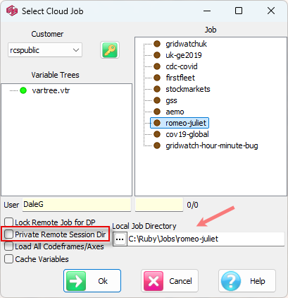
If checked, then reports will be saved in a cloud job's /Session folder which is private to the current user. This state is indicated by the cloud icon in the TOC tree.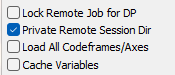
For cloud jobs, CaseData, Exec and User are always remote.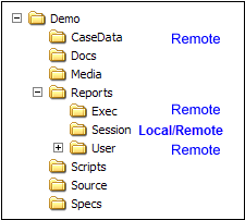
The job directory holds the job.ini file and any *.vtr (Variable tree) files.
CaseData holds the raw case data and meta data files.
Docs holds any files that have been added to the TOC as Document nodes in the Session branch. Document nodes in the User and Exec branches are stored in those sub-directories.
Media holds any pictures on charts or files attached to callouts. These are uploaded or downloaded with reports that contain them.
Reports has three subdirectories for Session, User and Exec reports. The TOC structure for User and Exec exactly mirrors the disk directory structure. The Session TOC bears no relationship to the directory structure except that all tables and charts are under the Session directory somewhere.
Scripts holds JScript and VB scripts. Ruby always opens browsers for these on the local drive.
Source holds source data files that are converted to Ruby case data by the Import processes. A remote setup usually has nothing here because you can only import to a local job.
Specs holds saved table and chart specifications on your local drive.
If Visual Studio is used, then there will be a VSX directory that will hold the VB.net program and all its supporting files.
Defining a Default Job Configuration - Job.INI structure
The default job.ini file is located in the Ruby folder where Ruby.exe is located. This file is can be used for any new job that is created.
This is a sparse job.ini file that can hold the standard colours, default base etc. for setting up an agency standard.
Most users find that the provided default job.ini file provides all that they require for a new job, however it is easy to customise this file for specific agency-wide job defaults.
The structure of the job.ini file is transparent and you can edit this file in a normal text editor.
Following is a discussion of the sections in the file and what you might want in a template version of job.ini.
Most of the job.ini content is set by your entries to the Preferences form.
The easiest way to identify how to describe your favourite settings is to organise them in a standard job and inspect the job.ini file.
You can leave out whole sections that are of no interest.
[Status]
DateRules=EU 4YYYY
You might want to set up standard date rules.
Hidden JobINI flags can be added to the [Status] section in order to control very specific behaviours - not in general use for all Ruby users, hence they are hidden from the GUI and can only be added via the job.ini file.
Often a job will be created using the default job.ini, then later the specific job.ini file for that new job can be edited to turn on/off the hidden functionality controlled by the flags.
[Imports]
Leave this out - each job will have different imports.
[PrintSet]
You might want to set up standard print settings.
[DefaultSeries]
Name=1
Color=0000ff
LineStyle=Solid
AbsWidth=333
Density=50
Dash=8
Marker=Circle
AbsMark=0
FillType=Solid
AbsBarPic=3333
PatWeight=50
BarPicture
Here is where you set up your standard series colours. Each of these is a block starting with “Name=n” and ending with “BarPicture” although you can leave out any parameter that is not of interest. Color is in hexadecimal pairs in the order Blue, Green, Red. The simplest approach is to set up the colours in a standard job and copy this section.
[TextMatchSeries]
Name=Execution1
Color=bbbbff
LineStyle=Solid
AbsWidth=333
Density=50
Dash=8
Marker=Circle
AbsMark=0
FillType=Solid
AbsBarPic=3333
PatWeight=50
BarPicture
This is a similar section to the previous but instead of “Name=” having a number, the name is the text that will trigger these cosmetic settings when it is found in a legend.
[Templates]
Table=TableTemplate
Chart=ChartTemplate
Spec
Base=cwf
The template table and chart is an alternative way of providing standard colours. New reports look first in these template reports then in the standard colours defined above, finally checking legends for text match if not turned off.
[Settings]
PadHierarchicData=1
ExcludeNE=0
InitTableAsMissing=0
KeepTabCht=0
You might have preferred settings here that all jobs should have.
[CodeList]
BrandX=1/3
BrandY=4/6
BrandZ=7/10
There might be some standard codelists that all jobs should have.
[SwitchFilters]
Males=GEN(1)
Females=GEN(2)
There might be some standard switch filters that all jobs should have.
[DrillFilters]
Males=GEN(1)
Females=GEN(2)
There might be some standard drill filters that all jobs should have.
[Favourites]
ChiSquare Test=@ChiSqrTest.jav
&Font Size=@Fonts.vbs
There might be some standard scripts that all jobs should have.
[AllowPercents]
Bases=1
#sum=1
#cmn=0
There might be some extra 'allow percent' behaviour you want in all jobs. Normally, in the Specification Form, when you drag codes to the Top and Side panels, codes get a percentaging mark (unless the variable is flagged as “No Code Percents” in the Variable form under the DP tab) and nothing else does. This section gives finer control over that.
The example shows you can change the general rule for codes, stats and bases (the defaults are codes=1, bases=0, stats=0) and make specific rules for classes of expressions. Any line starting with # applies to all expressions (blue dot functions, red dot arithmetic) plus brown dot bases and green dot stats. Any such line expression that includes the text after the # will trigger the rule.
The example shows a variable with a 'sum' arithmetic that was automatically percentaged, a 'cmn' arithmetic that was not, and when 'Base First' was employed the base was percentaged.
The full syntax currently available to AllowPercents is:
Codes=1 or 0
Stats=1 or 0
Bases=1 or 0
#XXX=1 or 0
... where XXX can be any text that might appear in an expression, base or stat.
[DecimalsFor]
#sum=1
#cmn=2
#avg=3
#tot=5
There might be some decimal rules you want to employ. This is similar to AllowPercents for setting the decimal places for different expressions, stats and bases. There are four switches on the Table Properties|Cells tab for setting general decimals for Frequencies, Percentages, Expressions and Statistics. This gives finer control after that.
[Imports]
DataChar=ANSI (Import File Character Type)
This is more a safety feature for the Card, Delim, SSS and SPS imports where the files could be UTF8 or ANSI.
UTF8 is generally a safe assumption but there is one circumstance that can be a risk: if the data collection software allows through a non-ASCII character. Page 2 characters (e.g. á) make sense as ANSI but not as UTF8.
When UTF8 is assumed, under Vista the character is replaced by another, but under XP the character is removed and the rest of the line displaced.
For a spec file this doesn't matter but for a data file the rest of the line will now be in the wrong columns.
If you know your data file is ANSI and not UTF8 you can assert this in job.ini.
[Imports]
Name=TestSSS
Type=SSS
DataFile=$SourceSSSTest.DAT
SpecFile=$SourceSSSTest.xml
DataChar=ANSI
SpecChar=AssumeUTF8
The DataChar and SpecChar lines can be inserted to assert the character type to expect.
SSS Data files are assumed to be UTF8 by default.
SPS Data files are assumed to be ANSI by default.
Hidden Job.ini Flags
There are some hidden flags which can be entered in the [Status] section manually to provide control over very specific functionality, as requested by some clients. These flags might be visible in the GUI sometime in the future, but so far have just been created to deliver special functionality as circumstances arose. The Boolean flags can be added to the Job.ini [Status] section as xxx=1 or xxx=0 where 1 = True and 0 = False.
Allow1x0Temp: for function expressions: Normally we don't want 1*0 in temp constructions because they add to the base. When zero is a legitimate code you do want 1*0.
BlankSubstitute: = your value to designate missing data
IgnoreCaseCounts: suppress the different case counts check for tables/constructions
IgnoreWeightWarning: don't bring up warning dialog if weighting stops before reaching the convergence limit
MDDImportLongestNames: MDD/DDF import uses long names for hierarchics
MeanSigBaseCounts: ignore Headcount stat setting and always use base (reproduces old behaviour)
ShowAxisLocks: show/hide the axis lock switches on the spec form (Silver only)
ShowCaseFilter: show case filter on spec page (Silver only)
ShowSigAsBkClr: Indicate significance by cell background colour
ShowSigBold: Indicate significance by bolding the cell font
ShowZeroP: Significance display for p=0 as blank or '0'
SkipBaseLimit: on the Significance tab is 'Ignore Base < 30' - change the limit from 30 here
TableauDataExport: BayesPrice flag for Delim exports to produce three files 'Codes ', 'Labels ', 'Meta '
TryAzureTemp: Azure caching: Look for cust_job_var.cd file in d:local emp, ... initial copy from blob if necessary
TTestZSwitchLimit: in TTest calculations switch to Z test when degrees of freedom exceeds this value (default 100,000) to roughly match decimal places accuracy.
TreesDescOnly: in trees the variable/axis name is suppressed if there is a description
UseOldRimWeight: Fast rim was introduced in Feb 2020 but old routine kept for legacy
These are turned on by =1, and off by =0, or by setting an appropriate value. Open Job.ini in a text editor an enter items as shown below.
With ShowSigBold=1 all tables with single cell significance show significant cells in bold:
Job Access Configurations
The following pages explain the job access configurations for:
Local Machine
Exclusive LAN
Shared LAN
Shared LAN, LAN Session
Local Machine
All files are on a standalone computer.
The Exec and User sections are on the local machine and can be used as a backup or organizing device.
Standalone users would normally run with the Exec and User sections hidden by turning the switch at File|Preferences|User OFF.
Exclusive LAN
All files are on the LAN. The user selected “Work Directly on LAN” when selecting the job.
This locks the job so no one else can use it until this user has finished.
This is handy for doing DP work such as a job update directly on the LAN, and for jobs that mostly have just one analyst.
The main advantage is the automatic backup via network procedures.
Shared LAN
Session reports are on the local machine, where the analyst explores things and organizes reports for sharing.
The User and Exec sections are on the LAN.
The idea is that the local machine Session section is a scratchpad where ideas are explored.
Each user has a named section on the LAN where shared reports can be uploaded (by dragging) and the Exec section is where completed reports for executive review are placed (this is the only section visible to an Exec user type).
The user had “Work Directly on LAN” checked OFF when selecting a LAN job.
Shared LAN, LAN Session
If you want all files stored on the network in a shared arrangement, you select LAN Session Folder.
Each User's Session section is now stored on the LAN.
Dragging Reports to User or Exec
When dragging reports from Session to User or Exec the files are actually copied onto the server (including any media they contain) so other users can see or take copies.
When you drag down to Session, from User or Exec, you receive a copy of the files on your local machine.
You can do this dragging in a Local data installation as well.
This now copies files into subdirectories on your machine and can be used as a way of preserving well-formed presentations or just making backups.
The Session section is thus always regarded as a 'scratchpad', with the User and Exec sections for more final work.
The User section is where different analysts can make available work in progress or store significant work.
The Exec section (the only one visible to an Exec logon) is where final presentations can be made available for Executive Information Services or Client access.
IT Setup Information
Users need read/write access to all job directories. Access to the program directory depends on the installation.
The Ruby directory minimally contains:
The program directory is also where other tools and documents would normally be stored.
The RubyJobs directory holds:
Ruby requires no OCX or DLL installations in the Windows or System directories. Last-run information is stored in the Windows registry.
Installation is simply a matter of copying the Ruby directory to the target machine.
Ruby requires online activation that can be done from the splash screen on first run.
The RubyDocs directory holds training, on-line help and reference documents.
Windows System Registration
For exports to MS Office and for scripting, Ruby.exe must be registered in the Windows System Registry. If you installed from setup.exe then this is done for you. If you installed from the zip then you will need to register Ruby.exe manually. This requires at least a temporary Administrator login to Windows. If you do not have Administrator privileges, then you will need to ask your local IT manager to do the registration.
From the Windows Start button
Run a Command Prompt as Administrator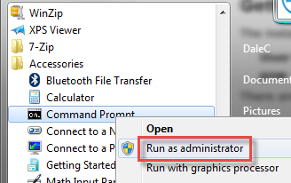
Navigate to where you have Ruby.exe installed. Type in cd Ruby. If you need to change drive letter simply type in the letter followed by a colon eg M:.
Enter Ruby.exe /regserver and press the Return key
You must see Administrator in the caption. There is no system response unless there is an error.
Moving Ruby
If you want move Ruby.exe to a different sub-directory after registering, you should unregister first to avoid duplicate entries in the system Registry. This is as above, but using /unregserver instead:
Then you can delete this Ruby.exe and register as above in the new sub-directory location.
Network Drives
If registering a network Ruby.exe, sometimes the Administrator mapped drive letters are not the same as the user letters - see
https://support.microsoft.com/en-au/kb/937624
The transparent fix for this situation is to map the drive twice to the same letter - once as the User, and once as Administrator. If in any doubt, ask your local IT.
After registering, Administrator privileges can be revoked.
Testing the Registration
In the Ruby Demo job (or any job), run or open a table and export to Excel
If Ruby is properly registered, and Excel is installed, the table will appear in Excel.
If you get any of these errors:
then either Ruby is not registered, or is registered incorrectly. This would be a matter for your local IT, since any number of things could be the cause.
Appendix 2: Internationalisation
File formats
Ruby uses UTF8 Unicode for maximum backward compatibility.
Unicode is a wide string text system with codes for every character in every language.
UTF8 is one way of encoding all of this so that the original ASCII character set is preserved without change (using one byte only) and other characters encoded with two to four characters as necessary.
With UTF8 there can never be any confusion between short or long sequences of bytes - previous systems gave garbled results if, for instance, one byte was dropped from a transmission.
Data import files are assumed to be UTF8 with a couple of exceptions:
SurveyCraft .SEQ files are assumed to be ANSI
any file with special leading characters (Byte Order Marks) will be recognised as Unicode or UTF8
Display
Displaying other scripts is always a matter of selecting the appropriate font and script.
The defaults for these are stored in the two templates (table and chart) for each job.
Entering text using non-English scripts requires controlling the font on edit fields and other Windows controls.
This is achieved with Ruby's System Font on the Preferences form.
A new installation of Ruby will initialise all of these fonts to your Windows Menu Font so in most cases the process is automatic.
System Font
Ruby keeps an internal System Font that is used for all its trees, lists and edit fields and the initial value of any new font.
This is initialised to your Windows' Menu Font so in most circumstances you will get the right script for your location automatically.
If you change it on the Preferences form the new setting is saved in the Registry.
To make charts from another location you can switch to that language by changing the System Font.
For instance, on an English machine, you can always see Polish charts properly because their fonts are stored with the chart but if you want to edit any Polish text you will need to switch System Font (and input language - but that's a Windows setting).
Otherwise you will not be able to type in the special Polish characters and they will not display properly in edit fields.
Switching Ruby System Font
Click the System button on the System Fonts and Colors tab.
You can select any font for the system font.
The important thing to check for non-Latin users is the Script.
Switching Input Language
Switching Input Language is a Windows setting.
After you have added other input languages in Control Panel|Regional and Language Settings|Languages|Details you can select them from the Language Button that appears near the System tray.
Templates
Preferences|Job Settings|Templates identifies a table and chart to be used as the template for any new ones.
If there are no entries for these then the fonts on new tables and charts will be initialised to Ruby's System Font.
As part of setting up the template reports you should make sure that all their fonts have the correct Script for your location.
In simple circumstances this should be automatic because new fonts are initialised to Ruby's System Font that is initially your Windows' Menu Font.
If you want to set up a template for another location you can switch to the System Font and clear the template settings in Preferences/Job Templates. Then a new table or chart will have all fonts copied from the System Font.
Fonts you cannot control
Some fonts are beyond Ruby's control.
The Captions on forms will always be in the font assigned in Control Panel|Display|Appearance|Advanced. You cannot change the script for those fonts.
When entering Edit Mode in a tree item by second-clicking it (slower than a double-click) you will be able to enter any text at all but it will be converted by Windows to your location script. On an English machine, if you are trying to give a Polish name to something then you will lose the special characters. To achieve this, you need a way of editing things other than second-clicking. Where there is not an edit field provided, you will find the right-mouse menu has a Rename item. This uses a dialog box that does preserve special characters.
Appendix 3: Processing Hierarchic Filters and Tables
For the avoidance of any doubt, this section shows exactly how table counts are derived from hierarchic case data. The case data examples are very small to make it easy to follow.
The point and value of hierarchic data storage and processing is that it obviates what would otherwise be a combinatorial explosion of variables. A classic example is a Brand/Attribute/Rating structure, which, with ten brands, ten attributes and a rating scale of 1 to 10, would require 10*10 = 100 variables comprising one only of brand, attribute or rating codes, or in the worst case scenario 10*10*10 = 1,000 variables comprising codes zero (no hit) and one (a hit for that rating for that attribute for that brand). Whether the cost is 100 or 1,000 depends on the system.
Hierarchic data storage allows such structures to be tabulated as if a single variable comprising multiple levels.
Level C
Single Response by Level C Hierarchy
SingFrwd.cd
1
2
3
4
5
6
BratRats is a typical brand/attribute rating hierarchy. The meta file BratRats.met looks like this:
[Codeframes]
(Brand)
1=brnd1
2=brnd2
(Attrib)
1=attrib1
2=attrib2
(Rating)
1=rat1
2=rat2
3=rat3
4=rat4
5=rat5
Each brand splits into two attributes, and each attribute is rated on a scale of 1 to 5.
Each respondent rates each brand for each attribute, so the data in BratRats.cd is completely rectangular:
Case#1: a1b1c1b2c2a2b1c3b2c4
Case#2: a1b1c4b2c3a2b1c2b2c1
Case#3: a1b1c1b2c1a2b1c5b2c5
Case#4: a1b1c1b2c3a2b1c2b2c4
Case#5: a1b1c2b2c4a2b1c3b2c5
Case#6: a1b1c5b2c4a2b1c3b2c2
The table with the group levels indicated is:
Because of the structure of the data in singfrwd, each column contains the data for a single case, with column#1=case#1, col#2=case#2, etc. Checking the first column against case#1, and splitting the case data with spaces to show the segment boundaries
Case#1: a1b1c1 b2c2 a2b1c3 b2c4
for the first block of ratings, a1b1c1 (that is, brand1, attribute1, rating1), the rating code at level C is code 1, so code 1 is hit once, and a count of 1 recorded in the top left cell. The second block, b2c2, hits code 2, so the count at row#7 (code 2 of block 2) is 1. The third block is a2b1c3, so code 3 at row#13 is counted once. The fourth block, b2c4, hits code 4, so the count at row#19 is also 1. In short, because the code frame has been contrived to have the codes at each level embedded in the labels, the segment aXbYcZ determines the row for brandX, attributeY, codeZ. The remaining columns are similarly verified.
Verifying the Table
BratRats by itself shows the totals for each row of singfrwd by bratrats arranged diagonally at the intersection points for each rating.
A second way to check this data is to compare to an unlooped or one dimensional version of the bratrats tree, and to add a totals column to the Top variable, SingFrwd. Because none of the codes repeat the counts should be identical.
This table is:
The values in the Totals column are the same as the diagonal values in bratrats by bratrats.
The unloop is done using the Line Generator.
A third way to check this data is to do the unlooping at run time by using nesting filters.
Brand.Rating nested on Attribute, then nested on Brand, produces equivalent output to singfrwd by BratRats except that the row headings show the defining filters instead of level names.
The specification is:
and the table is:
Using nested filters like this gives the same cell counts, but the percentaging bases will necessarily be filtered too.
Level D
The variable Exp (abbreviation for 'experiment') is a single case for a series of experiment outcomes such as testing a new pharmaceutical. The testing regime is organised into trials, which comprise sessions, in which the tests numbered 1 to 5 were conducted, and the result recorded. In this example, each laboratory conducts two trials, comprising two sessions, with any two of five different tests per session, duplicates allowed so that the same test can be run more than once.
The code frames for each level are
Trial
1= trial1
2 =trial2
Session
1=sess1
2=sess2
Test
1=test1
2=test2
3=test3
4=test4
5=test5
Result
1=pass
2=fail
The data for case#1 (the only case) in tree form is:
Reading the tree top down from left to right, this data says that:
Trial1, session1, test1 passed
Trial1, session1, test1 then failed
Trial1, session2, test2 failed
Trial1, session2, test2 then passed
Trial2, session1, test2 passed
Trial2, session1, test2 passed a second time
Trial2, session2, test5 failed
Trial2, session2, test5 failed again
If filtering to Trial(1), then only the circumscribed codes are candidates for tabulation.
The nodes for which Session(2) is true are enscribed. All processing under this filter is constrained to these nodes only.
Test(2) is true of the enscribed nodes only.
Result(1) is true for the enscribed nodes only.
Any level can be cross tabulated against any other level, any level can be cross tabulated against any other variable, and all levels can be tabulated against anything, with filters controlling the pools of candidate codes at each case.
Single Response by Level D
The table below shows the number of times each test passed or failed. The trees on the right show the paths to the leafs which are counted in the column of the table. The hierarchic structure of the data is represented in the nesting of the row labels and block headings.
Examples
The table Exp.Trial by Exp.Test will hit the cells (1,1), (1,1), (1,2), (1,2), (2,2), (2,2), (2,5), (2,5),
...to give the count of pair hits as...
trial1trial2
test1 2 0
test2 2 2
test5 0 2
Similarly, the table .Session by .Test will hit the cells (1,1), (1,1), (2,2), (2,2), (1,2), (1,2), (2,5), (2,5), to give
sess1 sess2
test1 2 0
test2 2 2
test5 0 2
That this is the same output as .Trial by .Test immediately above is pure coincidence.
The table .Trial by .Test filtered to .Trial(1) will hit the cells (1,1), (1,1), (1,2), (1,2) to give...
brnd1
rat1 2
rat2 2
rat5 0
The tree nodes for which .Trial(1) is true are free-hand enscribed. Crosstabulation happens ONLY within the enscribed region. The 'true' code .Trial(1) is circled, and its coordinate pairs are in the rectangle.
The table .Trial by .Test filtered to .Session(1) will hit the cells (1,1), (1,1), (2,2), (2,2) to give:
trial1 trial2
test1 2 0
test2 0 2
The tree nodes for which .Session(1) is true are enscribed.
The table .Trial by .Test filtered to .Test(1) will hit the cells (1,1), (1,1) to give:
trial1
test1 2
The tree nodes for which .Test(1) is true are enscribed.
The table .Session by .Test filtered to .Trial(2) will hit the cells (1,2), (1,2), (2,5), (2,5), to give:
sess1 sess2
test2 2 0
test5 0 2
The tree nodes for which .Trial(2) is true are enscribed.
The table .Session by .Test filtered to .Session(1) will hit the cells (1,1), (1,1), (1,2), (1,2), to give:
sess1 sess2
test1 2 0
test2 2 0
The tree nodes for which .Session(1) is true are enscribed.
The table .Session by .Test filtered to .Test(5) will hit the cells (2,5), (2,5) to give:
sess2
test5 2
The tree nodes for which test(5) is true are enscribed.
The table .Trial by .Trial filtered to .Result(1) will hit the cells (1,1) and (2,2) to give:
trial1 trial2
trial1 1 0
trial2 0 1
The tree nodes for which .Result(1) is true are enscribed.
Sparse Hierarchies
BrimRats is an example Brand/Image/Rating hierarchy across six cases. Unlike the Brand Attributes example (BratRats) the data is sparse, since not all respondents rate each brand or image.
The data for six cases is:
Looking just at case#1, the tree says that:
brand1 image1 was rated a 1
brand1 image2 was rated a 2
brand 2 image1 was rated a 3
brand2 image2 was rated a 3
The table SingFrwd by BrimRats shows the counts for each of the six cases in the corresponding column.
Examples
BrimRats.Brand by BrimRats.Imag
brnd1 brnd2
img1 5 4
img2 4 5
img3 1 2
Looking at the top row, for img1 only, the counts of 5 and 4 are derived from the tree by counting the number of (1,1) pairs on the left branch for brand 1 (there are five, at cases 1, 2, 3, 5, 6) and the number of (2,1) pairs on the right branch for brand 2 (there are four, at cases 1, 2, 4, 5).
The remaining rows are similarly verified.
BratRats.Brand by BratRats.Rating
brnd1 brnd2
rat1 2 2
rat2 2 6
rat3 6 3
Looking at just the counts for the rat2 row, 2 and 6, the derivation from the tree is...
There are two (1,2) pairs, at cases 1 and 3, and 6 (2,2) pairs, one at each of cases 2, 4 and 6, and three at case 5.
The table is symmetrical, giving
rat1 rat2 rat3
brnd1 2 2 6
brnd2 2 6 3
if specified the other way around.
BrimRats.Imag by BrimRats.Rating
img1 img2 img3
rat1 2 1 1
rat2 2 5 1
rat3 5 3 1
Looking just at the top row for rat1, the counts 2, 1 and 1 are derived from the tree as two (1,1) pairs at cases 1 and 3, one (2,1) pair at case 2 and one (3,1) pair at case 4.
The rows for rat2 and rat3 are similarly derived.
BrimRats.Brand by BrimRats.Rating filtered on Rating(2)
brnd1 brnd2
rat2 2 6
The enscribed tree nodes are true for .Rating(2), so only those nodes are considered.
There are two (1,2) pairs at cases 1 and 3, and six (2,2) pairs at cases 2, 4, 5 and 6.
BrimRats.Imag by BrimRats.Rating filtered on Rating(2)
img1 img2 img3
rat2 2 5 1
Only the row for rating 2 remains, and this should be the same as for the equivalent row in the unfiltered version of the table (see Ex 4 above).
There are two (1,2) pairs at cases 2 and 5, there are five (2,2) pairs at cases 1, 3, 4, 5 and 6, and there is one (3,2) pair at case 5.
Hierarchic Weighting
Any matching hierarchic level can be used for weighting. The examples that follow show this:
Example 1: BratRats.Rating by BratRats.Rating weighted on BratRats.Rating(*)
Example 2: BratRats.Rating by BratRats.Rating weighted on BratRats.Rating(1/3)
Example 3: BratRats.Rating by BratRats.Rating weighted on (sum_BratRats.Rating(*))>3
Hierarchic Weighting Example 1
BratRats.Rating by BratRats.Rating weighted on BratRats.Rating(*)
The unweighted table is:
rat1 rat2 rat3 rat4 rat5
rat1 5 0 0 0 0
rat2 0 5 0 0 0
rat3 0 0 5 0 0
rat4 0 0 0 5 0
rat5 0 0 0 0 4
...so weighting on BratRats.Rating(*) will multiply each column by its code number,
giving 5*1=5, 5*2=10, 5*3=15, 5*4=20, and 4*5=20.
rat1 rat2 rat3 rat4 rat5
rat1 5 0 0 0 0
rat2 0 10 0 0 0
rat3 0 0 15 0 0
rat4 0 0 0 20 0
rat5 0 0 0 0 20
Hierarchic Weighting Example 2
BratRats.Rating by BratRats.Rating weighted on BratRats.Rating(1/3)
Scope of the weights has been restricted to 1/3, so columns 4 and 5 get a weight of zero.
rat1 rat2 rat3 rat4 rat5
rat1 5 0 0 0 0
rat2 0 10 0 0 0
rat3 0 0 15 0 0
rat4 0 0 0 0 0
rat5 0 0 0 0 0
Hierarchic Weighting Example 3
BratRats.Rating by BratRats.Rating weighted on (sum_BratRats.Rating(*))>3
rat1 rat2 rat3 rat4 rat5
rat1 0 0 0 0 0
rat2 0 0 0 0 0
rat3 0 0 0 0 0
rat4 0 0 0 5 0
rat5 0 0 0 0 4
The weight expression is true only for ratings 4 and 5, and since true returns 1, the weight is 1.
This results in unchanged cell counts for (rat4, rat4) and (rat5, rat5).
This weight expression is equivalent to the filter BratRats.Rating(4/5).
Appendix 4: AutoUpdate of Ruby
The first time Ruby runs each day it will check for updates to system components.
The message Checking for updates will appear at the bottom of the splash screen and the action buttons will be dimmed.
If no updates are available, the message will go away in a few seconds and the buttons become active.
If there are updates, you are prompted to download them. You can decline but will be asked again.
If you accept, Ruby will initiate the download.
A companion program, RubyUpdater.exe (located in C:Ruby by default), checks for any files with version numbers and date stamps older than the current ones. If there is a newer version of the updater, then Ruby will download that first, and then any other files that need updating.
UpdateReport.txt is saved to the Ruby folder as a step in the update process. It contains the specifics of the updates applied.
Ruby will switch to the updater to collect new files.
After the update completes, UpdateReport.txt opens to display the changes to Ruby or other files, and a message box, saying “Click Ok to return to Ruby”.
You can run RubyUpdater.exe explicitly from its location in C:Ruby (or whichever directory you have chosen to locate Ruby.exe). You would do this if you knew there were updates available and you did not want to wait a day for Ruby to check automatically.
It is most likely your firewall will ask for permission for Ruby and RubyUpdater to access the Internet.
Click Allow or the equivalent button in your firewall.
Appendix 5: Excel Dashboards
Dashboards in Excel
The demonstration file is RubyJobsDemoDocsCustomDashboard.xlsm. This is a macro enabled workbook and you must allow it to run macros.
The CustomDashBoard is set up to run with the RCS Demo job.
Modifying for a different job, and for different sets of demographics, brands, measures or periods is easy and requires no programming.
The user selects a combination of demographics, the brands, a combination of measures and a period.
On clicking Generate Chart a simple macro invokes Ruby with Visible=false to supply the requested tables. Ruby should not be running - the macro starts/exits Ruby on clicking the Generate Chart button.
Survey series are plotted in the upper chart panel. External data series are plotted in the lower narrow chart panel.
You enter the path to your version of the Demo job at the cell D1 on the Home sheet.
Properties
Some properties will be reset by the macro at Generation time.
These are:
Lines series style for the upper panel chart if Period is anything other than count
Nested X axis and bar series on the upper panel chart if Period is Count
The chart title text is always concatenated from the three demographics
The Plot Area height of the survey chart expands or contracts depending on whether the lower panel for GRPs is present
Series width and series marker size are fiddly to change through the Excel GUI (because of the need to do each series individually) so the control panel on the right can be used to set width and size for all series on the survey chart. The marker size cannot be less than 2.
Any other chart property can be changed using Excel in the normal way. For example:
This gives a nearly complete control over how the charts appear.
Behaviour
The three demographic categories are ANDed and applied as a filter
The measures are plotted as indicated
If the period is Count (meaning the total period) then the lower panel is hidden and the style of the upper panel changes to nested X axis and stacked bars.
NB: Roll, Mark.Size and SeriesWid apply only to the upper chart panel
If the roll is greater than 1, then the first roll-1 data points (the roll-in) are suppressed
Marker size cannot be less than 2
Series width of 0 means you can change the widths manually - otherwise, 1 means thin, 2 means medium, 3 means thick
Editing the Categories
The framework for this dashboard is very flexible. Any user can change the drop-list items, the brands, the measures, the demographics and the periods by directly editing the Data sheet. You do not need to edit the macro itself unless more/less than three demographics or two measures are required.
As an example of the process, here is how to add more Age categories:
Two Age categories are defined, Under 35 and Over 35.
To allow the user to select any coded age band:
Select the Data sheet
Extend the Age entries like this
Back on the Home sheet
Select Developer | Design Mode
Right click on Age and select Format Control
Click on the Browse button for Input Range
Extend the selection as indicated
Click Close
Set the number of drop down lines to 9
Click OK
Turn off Design Mode
You can tell if you are in design mode or not by pointing to the Generate button.
If the mouse pointer is an arrow, then Design Mode is OFF.
The drop list for Age is now:
And selecting one of the ages, e.g. 15-25, shows on the chart title as:
All text in italics on the Data sheet supplies either a cell or a drop list text item on the Home sheet.
Customising the Charts
Select the chart
Use the Excel Chart interface to make changes to backgrounds, fonts etc.
If you want to make structural changes to the macro code then while developing it is a good idea to make Ruby visible so you can see what's going on.
Change True to False:
Save under your own name
Other Examples
For other Excel examples see
RubyJobsDemoDocsCustomSpreadsheetPull.xlsm
RubyJobsDemoDocsGenTabSpecsServer.xlsm
Appendix 6: Key Performance Indicators (KPIs)
Key Performance Indicators (KPIs)
The difference with KPIs is often that only selected bits and pieces of larger tables are required.
For circumstances where any arbitrary mix of inputs from Ruby and outputs to Excel is required, a useful approach is demonstrated in CustomSpreadsheetPull.xls - see RubyJobsDemoDocs. This uses a simple macro comprising two commands, CopyTable and CopyCell. CopyTable copies a Ruby table to a specified top-left corner cell of a specified spreadsheet. CopyCell does likewise, except that only a single Ruby table cell is copied. The copying uses the same flags as the Ruby API, and so is very flexible for things like row or column percents.
Testing the Demo
To see it all in action
Open CustomSpreadsheetPull.xlsx in Excel
Open SheetA
Note there is some commentary
On this sheet, only the cell values will be updated. The table labels will not be touched, allowing you to label the rows and columns in any way whatsoever. This gives the power to totally override the labels which would otherwise come from Ruby. The reason this happens is because the CopyTable last parameter is just “PercentSign”. The basic clip is cell values only. Everything else has to be explicitly requested via a concatenation of Copy flags. These flags are the same as for the Copy automation command (see Ruby Automation.pdf for details):
The parameters for CopyTable are:
CopyTable , , ,
While on SheetA:
Delete some table values so as to mess up the chart
Open SheetB
Note the commentary
This time, the labels will be copied along with the cells.
Delete some table values so as to mess up the chart
Open SheetC
Note the commentary
The CopyFlag TopGroups prevents the legend text from becoming too verbose. If you want all nested levels of labelling, use just Groups.
Delete some table values so as to mess up the chart
Open SheetD
Here, the indicated cells are populated by a bank of CopyCell calls:
Open up the program by Developer | Visual Basic to see the details of the macros.
The parameters are
CopyCell , , , ,
The cell copy flags are:
Remove some of the percentages
Return to the Home sheet
Check that you have the job path c:RubyJobsDemo (or wherever)
Click the Generate Tables button
In a second or so all the charts and the percentages are updated with the correct data.
Sheet E gets a slab of numbers too.
Editing for your own KPIs
To adapt for your own KPI reporting regime, save CustomSpreadsheetPull.xls under a new name, and then edit the sheets and the macro code according to your requirements.
Appendix 7: Enhanced MS Office Documents
For full details, see Ruby Push Pull Reference Manual.pdf on the ribbon Help page.
Or open directly from RubyDocs.
Appendix 8: Statistics in Ruby
This section describes the statistics behind the Significance settings on the Properties form.
Headcounts
The 'n' used in the formulae for determining degrees of freedom and estimating variance using p(1-p)/n can be the Effective Base (if that switch is set), the Weighted Base (if that switch is set) or the unweighted headcounts. There will be no difference for unweighted data and for reasonable weights the difference rarely extends beyond the third decimal place.
Effective Base
Headcounts are 'effective base'.
eb = (∑w)²/∑w²
where w is the weight for a particular respondent.
Weighted Headcounts
Headcounts are weighted (ie cwf) rather than unweighted (ie cuf).
Variance Options
Estimating variance for a proportion is essentially v = p(1-p)/n.
When two proportions are involved there are two approaches to estimating the combined variance:
Simply sum the variances
or start with a pooled proportion
The second approach is more common in hypothesis testing. The null hypothesis is that the two proportions are coming from the same population so a better estimate of the parent population is gained by combining the samples.
Default - Pooled Variance
Use Pooled Proportion for Variance Estimate
Adjustments for small sample size are added to exactly match Quantum.
Use Overlap Formula for T-test on Proportions
For a multiresponse variable where each person may contribute to many columns you can apply a modifier that adjusts the variance to account for the overlap cases.
The variance is modified with a covariance term
where n0 is the overlap headcount and r0 the correlation coefficient
where f1,2 are the frequencies for the cells, f0 the overlap frequency and n0 the headcount of overlapping cases.
An example of this formula can be found in the Quantum documentation volume 3 p180 - but note there is an error in the correlation coefficient there: they have p0,1,2 in the formula instead of f0,1,2. (Confirmed by SPSS).
Degrees of freedom is adjusted as
Use Continuity Correction
Tests of Proportions
All tests produce a statistic
or
with the continuity coefficient.
Variance is determined according to the option settings.
For a t test, degrees of freedom is
Single Cell
This tests the proportion in the cell against the 'rest of the table'.
x=cell, r=rowbase, c=colbase, t=corner
Cell proportion is p1=x/r. The rest of the table proportion is p2=(c-x)/(t-r).
For t tests df = t-1.
Cells are coloured to indicate three levels of significance.
To exactly reproduce results from SurveyCraft:
? Z Test
? Use Pooled Proportion for Variance Estimate
✔ Use Weighted Headcounts
Row/Col Groups
A parameter string indicates which rows/cols to test against each other. e.g. abc;def means test a, b and c against each other and independently test d, e, and f against each other.
Significance is indicated by letters in the cells.
The larger of a pair that are significantly different.
e.g. 'Ca' in a cell indicates it is significantly different to (and larger than) rwo/column 'C' at a high level of significance and row/column 'a' at a low level of significance.
To exactly reproduce results from Quantum:
? Column Groups
? T Test
✔ Use Effective Base
✔ Use Pooled Proportion for Variance Estimate
✔ Use Overlap Formula for T-test on Proportions (as necessary)
Reference Row/Col
The first row/column is used as a reference and all other rows/columns are compared to it. Significant cells have colored text depending on the level of significance. These tests use typical adjustments to variance estimation so will be slightly more conservative than the single cell test.
Tests of Means
The only rows/cols recognised as means are the standard stats AVG and CMN for which the standard variances VAR and CVR are available. The statistic is (z or t):
There are two choices for estimating the variance and degrees of freedom.
Summed Variance
For a t test, degrees of freedom is
Pooled Variance
This is the method employed in MColumnTTest.js
The statistic is
... but the variance is more sophisticated.
The effective headcount for each sample is
.. and the effective base is
Then the variance is
... which, for unweighted data reduces to
... and the standard error is
For a t test, degrees of freedom is
Appendix 9: Ruby's Data Flow
This section describes the data flow and interface connections between Ruby and the outside world, and the flow inside Ruby from Variables to Reports.
Data Sources
Ruby can import directly from many of the major data sources:
SPSS .SAV
SPSS .SPS
UniCom Intelligence Data Collection .MDD and DDF (Dimensions)
SSS DataMap XML
SSS multi file XML levels Datamap
Quantum Runfile and Data
SurveyCraft
Delimited ASCII
Fixed-width ASCII
Another Ruby job
There are several tools and techniques for importing almost any form of ASCII data.
Ruby expects clean source data and there are a variety of tools provided within Ruby to identify and remedy data issues.
Most often data cleaning is performed by the data collection team, within the collection software, and this exported clean data is used as the source for a Ruby import.
Data Exports
Ruby case data can be exported in a variety of formats for import into other analysis programs:
SSS 1.2 .XML Map Fixed-width ASCII .ASC
SPSS Syntax File .SPS, Fixed-width ASCII .ASC
SSS 1.0, SSS Map, Fixed-width ASCII .ASC
SSS 1.1 SSS Map, Fixed-width ASCII .ASC
SSS 1.2 XML Map, Fixed-width ASCII .ASC
SurveyCraft .PRN Map, .SEQ Data
Delimited Data, .CSV, .TSV, or .SSV
Ruby can deliver presentations and include any document type (as a virtual shortcut) in its table of contents. In this way Ruby can be used as a repository of all data, knowledge and information about the job.
Presentation exports are available to explicit Microsoft products (PowerPoint, Excel and Word) and to general data and image formats.
Since Ruby uses Windows' own automation language it can communicate with any other such program (like Excel, PowerPoint, Word) for routine or customised exports.
Internal Data
This diagram shows the flow of data from case level variables to the raw cross tabulations which provide the data displayed in reports.
The expressions in blue are examples of the algebra available at each stage.
You can view in-memory raw crosstabs by a double-click at the Raw CrossTabs page of the In RAM form.
Raw Crosstabs
Reports are built in a two-stage process: simple raw crosstabs are generated and assembled according to the specification into a display.
Raw crosstabs have only one variable across and one variable down optionally with one filter expression and one weight expression.
The rows and columns are always a complete set of codes and pseudo codes for each variable.
This means every code, all standard bases and statistics (if the spec has at least one statisitc), and every pre-defined arithmetic code like c1+c2 in Age above.
Raw crosstabs are accessed via the In Memory form which shows all crosstabs currently in memory.
Selecting a crosstab and clicking OK (or double-click) displays the table as tab-delimited in a text window.
To see the figures in more detail, highlight the text, clip it with [Ctrl]-C or similar and paste it into a spreadsheet.
At generation time, Ruby checks the raw crosstab list to see if a required crosstab is already available. If not, then the raw crosstab is generated from scratch.
Displayed tables, charts and maps can draw from any number of raw crosstabs, pulling out only the cells of interest. It is possible to have display tables that need only one raw crosstab or ones that need a different raw crosstab for each cell.
Appendix 10: How Do I ... ?
Commonly asked questions and frequently used Ruby methodology are explained here.
Indexed Reports
Transfer a Ruby job
Specify a Table with Percentages on a Single Value
Confidence Intervals
Prepare a Ruby job for Laser
Indexed Reports
Indexed reports recalculate cells to dimensionless units above or below a normal such that all indices average to the normal. It is the relative size and above/below the normal that matters. The usual intention is to eliminate the “Brand Halo” effect. The classic example of a halo effect is Coca-Cola, which always scores highly on attributes because of its oversized brand awareness. The most common normals are 100 or zero. Indices close to the normal represent “Motherhood” statements - like every bank has ATMs, it is a given. Indices substantially above/below the normal are the discriminating categories. There are several ways to index a table, and which is best for any given scenario is an analytical decision.
If your Ruby setup installation file is later than December 2022 then the example reports can be found in the /Miscellaneous TOC folder of the Ruby Demo job.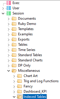
The reports are named for the index method and the axis variables. Each method is explicated in the following topics with reference to the relevant Index_* example reports.
Percent of Average
Column Percent of Base Percent
Subtract the Averages
Normalise by Standard Deviation
Scale from -1 to 1
Percent of Average
Report: Index_PercOfAvg_BIM
A common application for indexing is a brand image grid. The specification and runtime flags are
Set the base column to the row averages pseudo code avg by the variable right mouse popup menu.
The base and last columns as average is for diagnostics: each indexed row should average to 100, indicating that the index values for that row are equally above/below the 100 normal.
Generate and display with frequencies and row percents, as
102.7 = 100*7909/7748.5, etc.
Report: Index_PercOfAvg_BIM_Radar
For charting, the frequency rows and average columns are not needed. Remove from the specification and plot as a Radar chart:
BrandX is considered the best value for money, the least expensive and somewhat higher on quality and reputation. BrandZ is regarded as the brand used by professionals. Brands Y and Z are considered expensive and not seen as value for money. Respondents do not discriminate the brands on “Well known”, “Modern” and “Easy to get”.
A quick sanity check is to roll the chart at more points than are plotted. If correct then the series should converge to 100 at the last spoke (or column).
Report: Index_PercOfAvg_BIM_Avgs_Compare
A complication is adding a series for the average of the indices. Just adding an averages row delivers the average of the frequencies, not of the indices.
To add average on indices here an expression is needed. Using the avg# function or the avg pseudocode does not return the index average because the operands are the underlying frequencies.
The incorrect 99.50 is the row% as 100*6568.67/6601.83, but the average of the indices is (102.07+97.40+98.44)/3 = 99.3.
To get 99.3, and similarly for the other columns, we must use the expression (v2$r+v3$r+v4$r)/3 instead:
vN$r means the row percents at the Nth vector (and vN$c means the column percents). The last column c1%avg (meaning code 1 as a percent of the average) is a diagnostic to check the first image statement.
Report: Index_PercOfAvg_BIM_Avg_Radar
For a plot, turn off Frequencies, remove c1%avg column, remove the incorrect averages, remove the bases, add the expression ins#(#100) for the normal and then move the average expression to the top row (this is so that as an area plot it will be plotted first, underneath the line series).
Report: Index_PercOfAvg_BIM_Alt_Spec
As the c1%avg column in the Index_PercOfAvg_BIM_Avgs_Compare table shows, this syntax could be used as an alternative to vN$r. The table specification is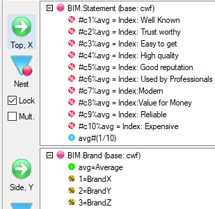
Since every cell is an arithmetic calculation, display as frequencies only:
Report: Index_PercOfAvg_BIM_Brand
This table does the percent of average on the brands instead of the statements.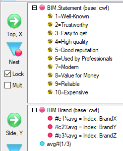
Reports: Index_PercOfAvgOfPercOfAvg_TP_BIM, Index_PercOfAvgOfPercOfAvg_SP_BIM
This is a double-index procedure. First, calculate the percent of average on one axis, and then use the results as the operands to the percent of average on the opposite axis.
These two tables have the same axes specifications but with different priorities - Top Priority on the left, and Side Priority on the right.
The second quadrant is the same as Index_PercOfAvg_BIM_Brand. The third quadrant is the same as Index_PercOfAvg_BIM_Alt_Spec. The fourth quadrant further indexes the second or third quadrants according to the axis priority.
The first three quadrants do not change according to priority (there are no expression conflicts) but the fourth quadrant behaves differently. For Top Priority, the fourth quadrant is the Brand index of the Statement index, and for Side Priority, the Statement index of the Brand index.
The calculations are
Column Percent of Base Percent
The index calculation is 100*(100*code freq/column base)/(100*row total/grand total), or, more abstractly, as 100*(column%)/(base%), that is, col% as a percent of base%.
Report: Index_ColPercOfBasePerc_BBL_EDU
The full specification and run-time flags are
Generate and display as row% only.
In the above table, the index score 88.15 for the cell (LT High School, Brand 1) is calculated on the category frequencies as follows (using 4 DP to minimise rounding):
The count table as frequencies and column percents:
Column% = 100*387/3032 = 12.7639%
Row total = 1448
Grand total = 10000
Base% = 14.48%
100*12.7639/14.48 = 88.148 = 88.15.
Note that since the base column is Totals, and Total is a statistic, Arithmetic Over Stats must be ON. Otherwise the Total takes priority, giving the sum of the calculated column percents instead, as
150.626 = 12.764+15.043+...
Preparing a table for this index procedure is somewhat fiddly, so there is a utility script which does it for you.
Copy and adapt to your requirements.
Report: Index_ColPercOfBasePerc_BIM
It is good practice to always show the average column as the right-most column to confirm that the rows average to 100, but this is redundant in the chart view.
To get the best of both, as below...
...set the radar chart's X axis high-bound to 9:
Subtract the Averages
This index method subtracts the row and then column averages from each cell. The normal is zero. Starting with Brand Image grid frequencies, the steps are
Column of the row averages
For each row, subtract the average from the cell
Convert to column percents of the base
Row of the column averages
For each column, subtract the average from the cell
If the calculations are correct then the indexed cells at a row will sum (and average) to zero.
Report: Index_SubtractAvg_BIM_Antecedents
This table shows an implementation of the above steps. The indexed cells are at the bottom right.
The specification and run-time flags are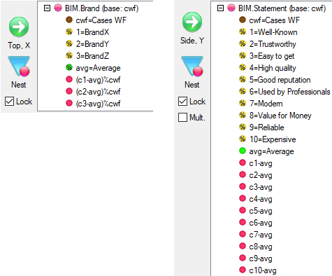
The run-time flags determine the evaluation priority order.
Report: Index_SubtractAvg_BIM
The antecedents (except avg) are not actually required, so the standard specification and table (retaining the optional diagnostics column) are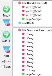
The avg vectors can be hidden by the right mouse pop-up menu.
Normalise by Standard Deviation
Report: Index_NrmFunc_BIM
This method is often used for scientific data. The normal is zero. There is a built-in function nrm# which does the work.
The specification and table are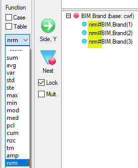
Scale from -1 to 1
All indexed categories are set to the same scale. Unlike the other indexing methods, this one does not average to a normal.
Report: Index_AmpFunc_BIM
Like nrm#, use the built-in function amp#.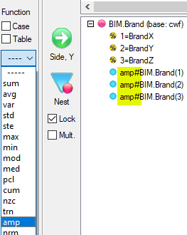
There will be a 1 for the maximum cell at a row and a -1 for the minimum, with all other cell values scaled proportionally in between.
Transfer a Ruby job
Overview
Ruby jobs can be transferred using normal file management tools. That depends on some knowledge about Ruby job directory structures.
Ruby includes zip/unzip tools that put all the files in the right place without having to worry about directory structures. The only requirement is that the source and target jobs have the same name.
Job Zip
You choose what bits of the job you want included in the zip - see Archive Group for more information.
The Zip field is filled with a default name built as . You can change the name.
Job Unzip
Job name must match. This must be going into a job of the same name or Ruby will not unzip. This is a safety measure so you don't put the wrong data in a job.
Creating a new job: If this is the first zip for a new job the receiver will need to create the job first.
Analyst users can create the job manually: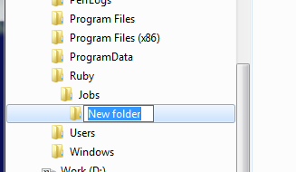
Just create a new folder where you want the job to be and name it to match the job from which the zip came.
Then open Ruby and select that folder as the current job.
There's no Vartree to select yet so you'll get this message.
Click Yes to confirm and all the job directories will be created.
Specify a Table with Percentages On A Single Value
Open the Ruby Demo job
Specify the table BYREG by BBE with Case bases both ways.
The point of this is that both variables are multi-response, so the top left corner will not be the number of respondents. It will be either the sum of base values in the horizontal or vertical directions, depending on the priority setting.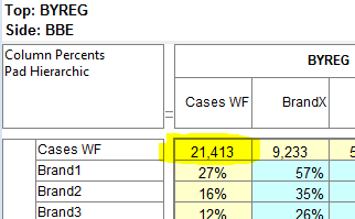
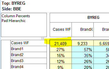
If you now set the top left corner to weighted filtered respondents:
The top left cell becomes 10,000:
To percentage all cells on 10,000:
You could just insert #10,000 as the base, but then if the table is filtered, the base will be unfiltered.
In the meantime, the work-around is:
Set base priority to Top
Respec and add a Count column with base as cwf
Set the local base for BBE to @cel#(1,0)
The table should appear as:
You can then hide the Cases WF rows and columns as desired.
It is intended to make percentaging on a single table cell a table property in a later version of Ruby.
Set Confidence Intervals
Overview
To get confidence intervals requires implementing v=p(1-p)/n.
The Data
The essential variable is AveRead_MF_443 which records readership with decimal codes.
The question was 'how many days do you read a particular paper?'
The number could be 0 to 5 and the construction scales this to 0 to 1 with decimal codes, so it effectively represents 'proportion of week this paper is read'.
The variable is single response.
Target Report
First Principles
This specification explores the variable.
Looking at the total column, 35551.39 people didn't read the paper at all, 56.12 read it 20% of the time etc.
These numbers can be put into Excel so the calculation can be built from first principles.
The x and f columns represent the data from the Ruby table. 0.2 occurs 56.12 times etc.
The following columns build up intermediates for mean and variance calculations. xf is column x times f, xxf is column x squared times f.
Row 11 is the sums of the columns above (note the 91.114 in the xf column, which is the 91 from the Target Report first column).
Applying standard formulae calculates the following:
Mean:
Variance:
Standard Deviation:
Standard Error:
95% Confidence:
Note that the mean for this variable is 0.024559 - which is the 2.5% readership of the report table.
However, this won't appear as a percentage in a Ruby table.
In column F all the stats in the column have been multiplied by n (same as total and cwf) to give the frequency numbers you need in a Ruby table.
In Ruby
So, in Ruby, cmn and cse will give the actual percentages required.
...but these are frequencies and we want those numbers as percentages.
Each needs to be multiplied by the appropriate cwf.
There are several ways to do this but the neatest is to put those in as arithmetic expressions.
Click Arithmetic
Type cmn*cwf (could be done by drag drop but quicker to just type)
Click OK
Back in the Variable form change the Label
Repeat for cse*cwf*1.96
Close Variable form accepting changes
Now they can be tabulated and percentaged.
...gives this table ...
... showing total readership is 2.5% +/- 0.4% at 95% confidence.
SE for one code of a conventional variable
Another variable type is like this:
Readership is defined as the percentage of code 1.
The issue now is to calculate the 95% confidence intervals for the single percentage 1.62.
The usual method is
Standard Error:
95% Confidence:
This can be entered as an arithmetic expression in a codeframe, and to appear as a percentage, we can use the same device above - multiply by cwf as well.
In Ruby syntax this is:
1.96*cwf*((c1/cwf)(1-c1/cwf))^0.5
You have to use c1/cwf for p, making the expression bulky.
The minimal character simplification after some algebra is:
1.96*(c1-c1*c1/cwf)^0.5
In similar fashion to above add an arithmetic node to the variable and use it in specifications.
Remember to double click the node to toggle percents.
Prepare a Ruby job for Laser
The TOC Tree
The Table of Contents panel in Laser is built from the Ruby Exec and User sections.
The other navigation displays show reports available to the current user only (excludes other users but not Exec).
Exec Section = Common Reports
The Exec section from Ruby appears in Laser for all users no matter what display.
For the User tree, Exec is renamed as Common.
In the Accordion display the Exec folders appear as if they were User folders.
The Exec section in Ruby is for common reports that everyone can see but no one can overwrite. Exec reports are maintained by DP and uploaded at each job update.
Vartree and AxisTree
The Vartree and Axis trees in Laser are identical but there's more customisation available in Laser - see below.
If you need things like local filters and weights or extra base types or custom expressions, then define and save in Ruby desktop and expose via the Laser Axes tree.
Some jobs use axes for everything and leave the vartree blank.
Drill & Switch Filters
The Drill and Switch lists are the same in both.
Tables
No vertical text
Ruby reports support vertical text but Laser ones do not. Ensure label widths are adequate for readability.
No Text Align Control
Ruby handles text aligning better, especially Middle aligned. A good compromise is to align to top.
Charts
No Pictures, Text or Callouts
In Ruby you can add pictures, text and callouts. These are not transferred to Laser.
Considerations
Vartree/Axestree
Clean and Lean
The Vartree (and AxisTree if you are using that) should be as simple as possible to serve the analytic requirements of the intended audience. Remove any source or DP variables that are not part of direct analysis, especially administrative variables like interview start/end times. These can remain in the Casedata directory but should never be exposed by a Laser variable tree.
No Case Variable
Typically, you would not want to expose data at the case level so make sure to remove the Case or other Respondent ID variables from the vartree.
Custom Trees
In Ruby you can make many vartrees saved as different .vtr files, but there's only one axis tree in Axes.atr.
In Laser you can organise a custom vartree and/or axis tree for each logon. The sequence Laser uses when someone logs on is -
For vartree:
Look for .vtr
Look for RubyLib.vtr
Look for RubyWeb.vtr
Look for RubyCom.vtr
Look for Vartree.vtr
And for Axis tree:
Look for .atr
Look for RubyLib.atr
Look for RubyWeb.atr
Look for RubyCom.atr
Look for Axes.atr
So you can set up individual trees for particular users. To send all the trees use the All switches on Job Zip. It is always best to have the default RubyLib version there as well, so nobody ends up with an empty vartree.
Drill and Switch Filters
Drill filters should be simple and germane. Remember these are progressively ANDed and can be undone so supply a set that covers your users' needs without being too many.
Switch filters should be a different list. These are not ANDed but apply individually - each new selection replaces the previous. They should represent well defined segments of interest and are likely to be more complex that the drill set.
There should always be a Switch 'None' option for removing the filter altogether - but not a Drill 'None' option because appending nothing is pointless.
Axis Locks
In Ruby you can choose to Lock axes or leave them unlocked.
This affects what happens when a report is Updated after a new data import.
If the axis is unlocked then any new codes will be added to the axis. This is good if you want each new week or month to come in automatically as a new row/column/legend. It is not good if you have selected just a few codes from a big brand codeframe - the update will pull in all the other brands as well on the assumption that they are new to the current wave.
So, Locked means do not add new codes as new rows/columns automatically.
In Laser, a new table is always given Locked axes. This is a safety measure because in Laser, reports are always updated invisibly when new data arrives - and you don't want them adding more rows/columns.
Laser users can change Lock status on Laser's report Specification/Edit form.
Users
User access will be managed by desktop tools that allow adding jobs and users. User permissions can be set to range from allowing simple viewing ability to full table creation, edit and export.
Global Filter
Each user can have associated a Filter that acts as a global filter on all data so that one set of reports can serve as the source. A typical scenario is a global job where analysis is always regional, or to restrict case data access to particular users for security reasons.
Reports
Laser will handle big reports faster than most online environments, but it will be slower than the desktop. Try to avoid large and complex reports. You might break into smaller reports something like a comprehensive summary that is instant on the desktop but might have a few seconds delay online. Use Dashboards to convey quick information like KPIs.
Job Update Process
Ruby Job Zip
Laser will only read a zip file prepared by Ruby and it must be from a job of the same name.
Once everything is ready use Ruby's JobZip form to prepare the upload file.
You do not need to have all the switches set. If you only want to send reports you don't need the Job.INI, Vartree and Casedata switches on. Only send what has changed.
Job.INI includes the Drill and Switch filters
Vartree.vtr is the list of variables exposed in the specification form
All - if you have multiple custom vartrees send them all
Axes sends Axes.atr
All - if you have multiple custom axis trees send them all
Case Data is the raw data as CD and MET files
Templates is the table, chart and spec on Preferences/Job Settings
Exec sends the Exec section for common reports visible to all
Users holds the reports - toggle users on/off to select them
When you send User folders the set of reports is merged with the existing set so no client-side reports will be lost.
Laser Job Update
This opens a file dialog - navigate to the zip file you just created in Ruby and click OK.
The zip will be uploaded, unzipped, deployed and the job display refreshed.
For more details on updating a Laser job see the Laser on-line help.
Appendix 11: Command Line Interface
There are three CLI flags:
Script=
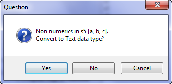

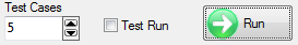
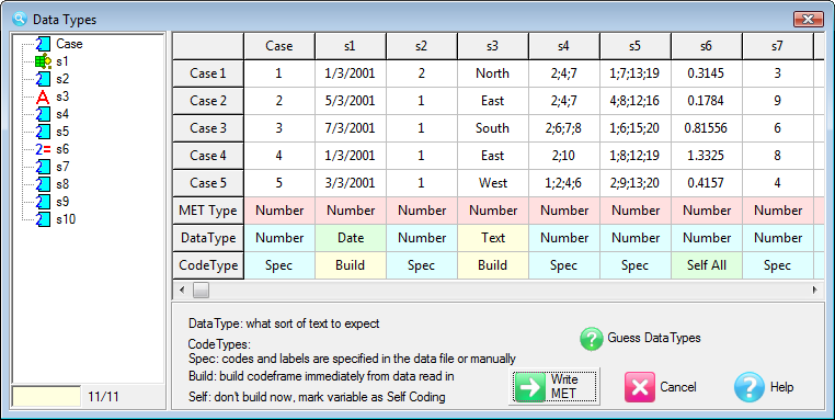
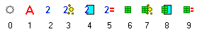
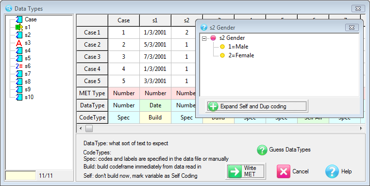
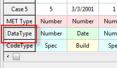
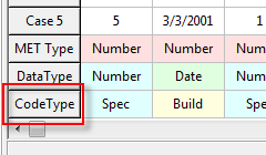
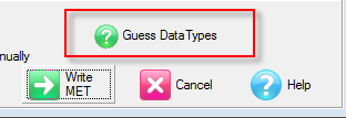
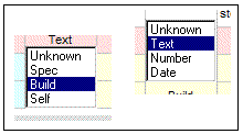
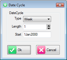
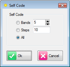
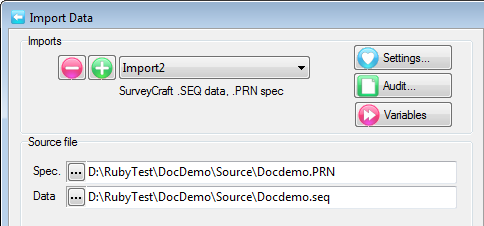
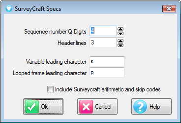
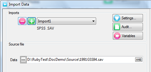
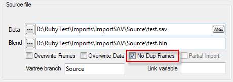
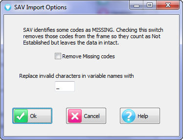
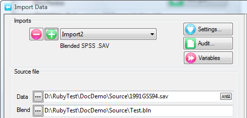
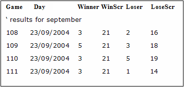
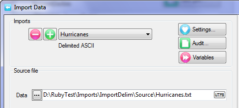
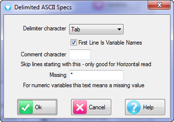
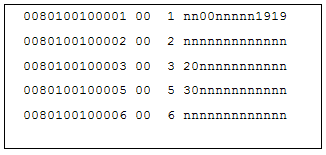
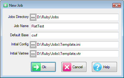
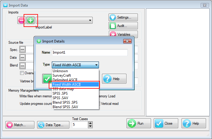
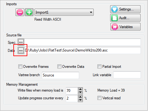
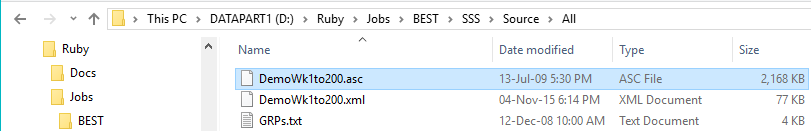
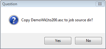
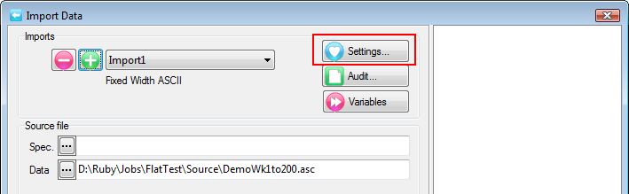
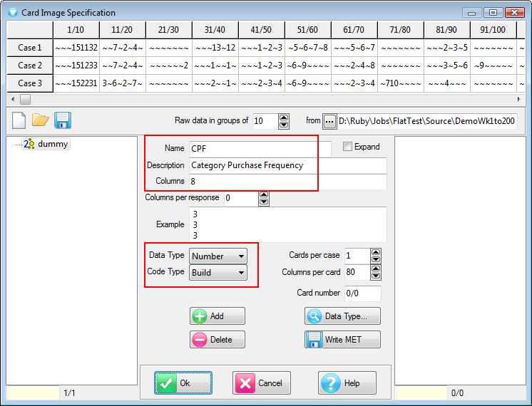
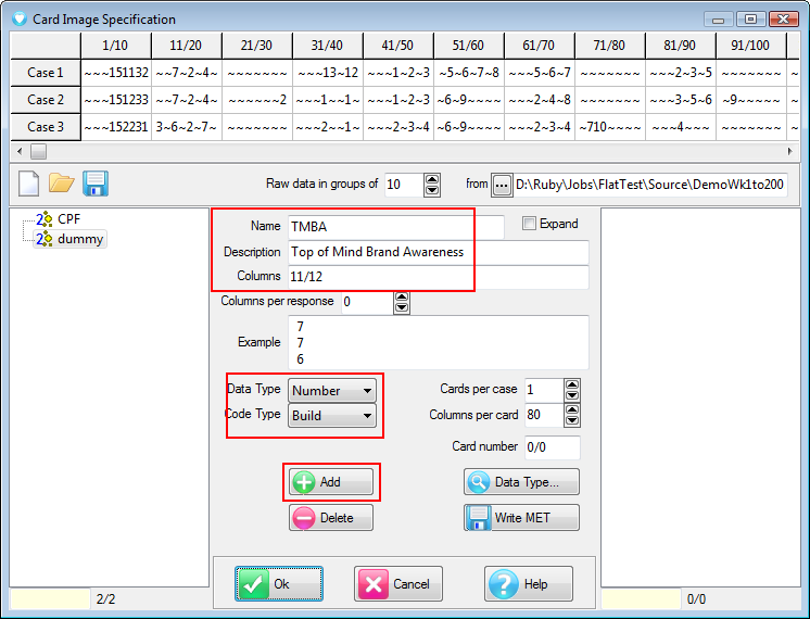

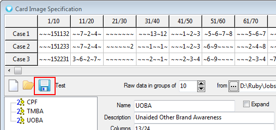

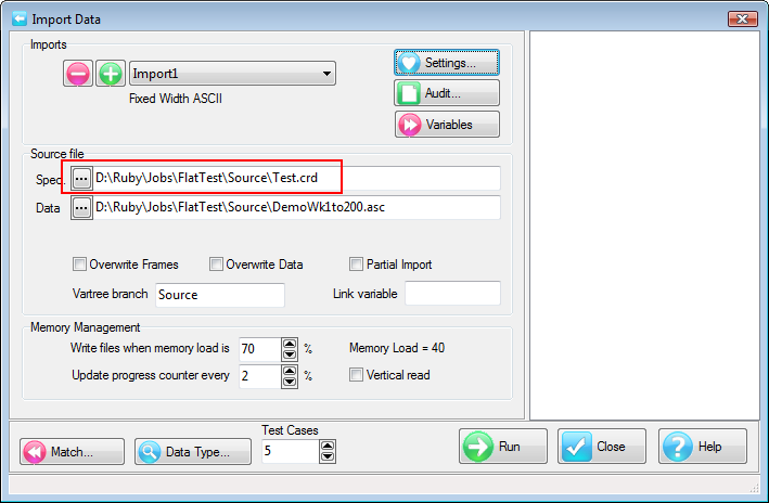

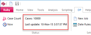
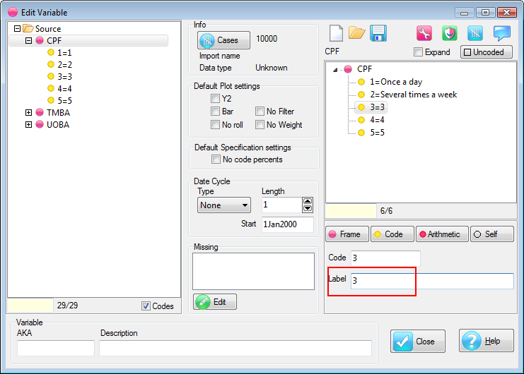
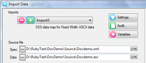
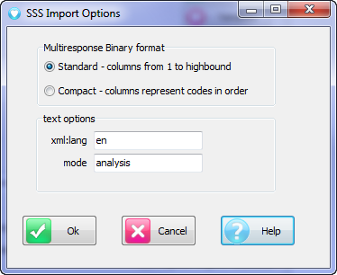
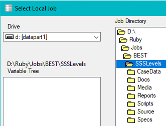
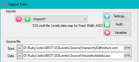
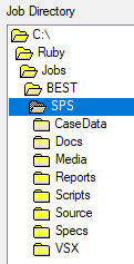
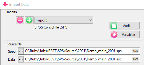
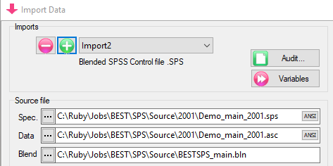
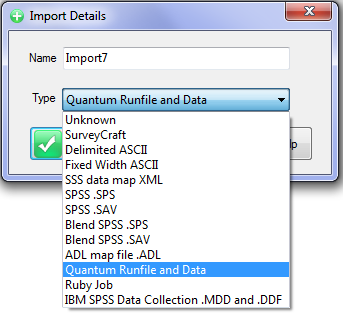
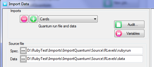
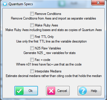
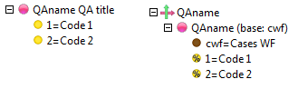
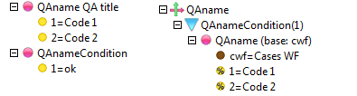
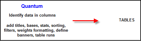
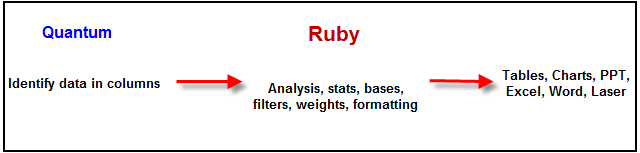
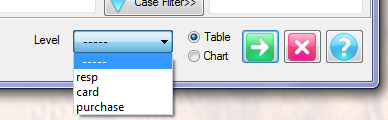
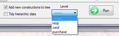
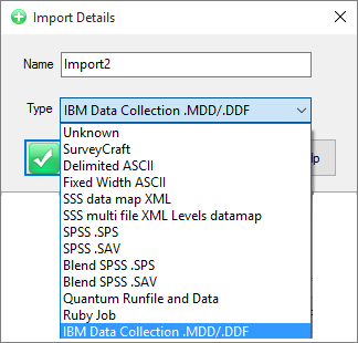
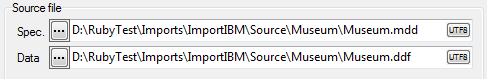
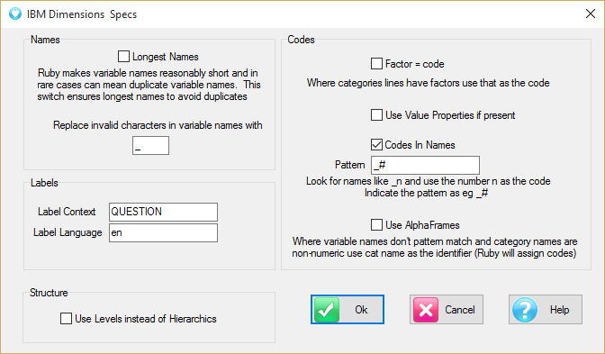
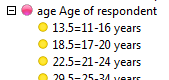
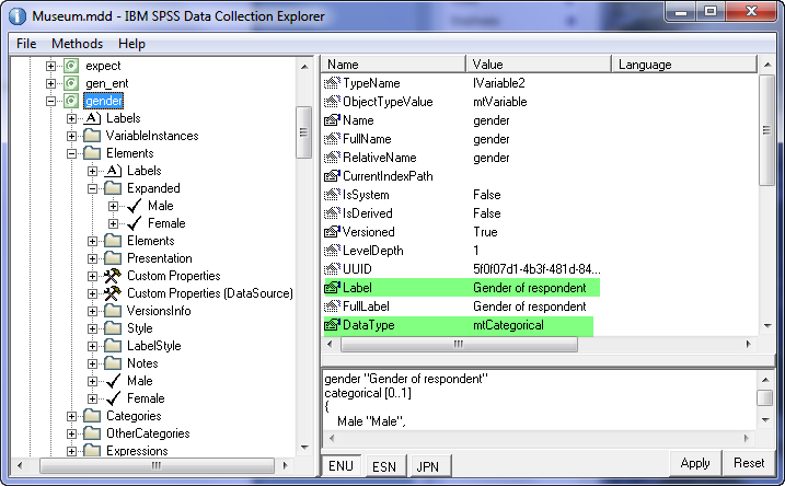
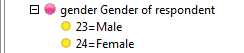
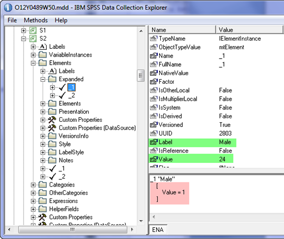
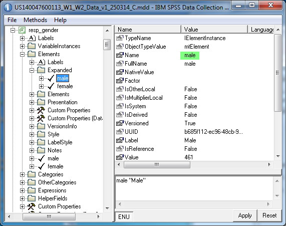
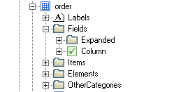
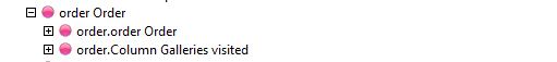
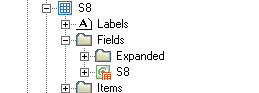
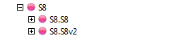
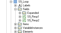
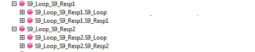
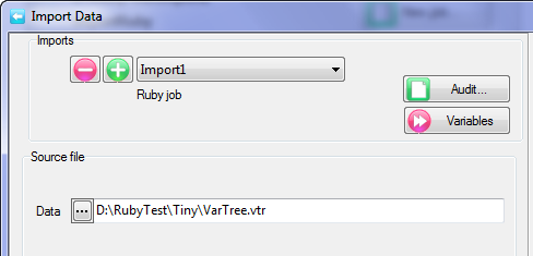
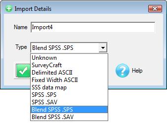
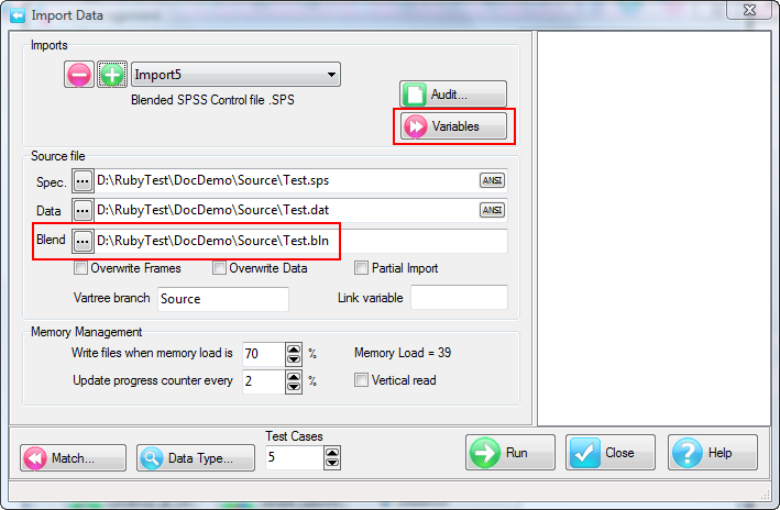
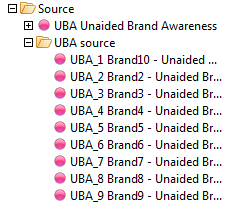
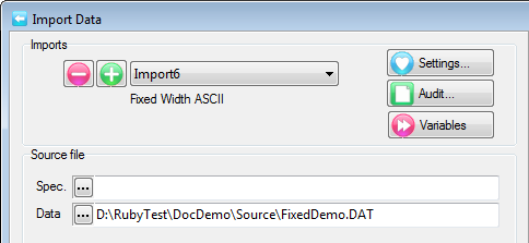
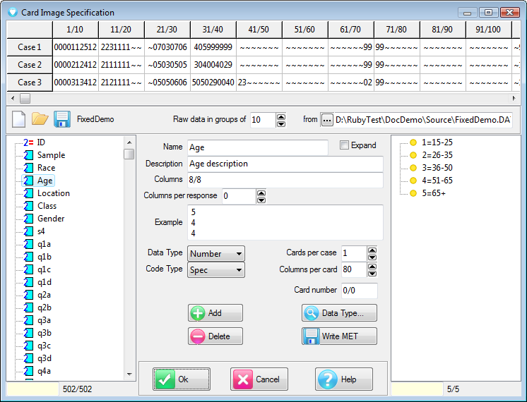
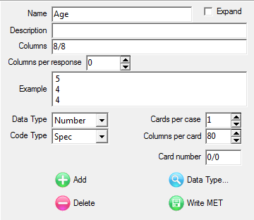
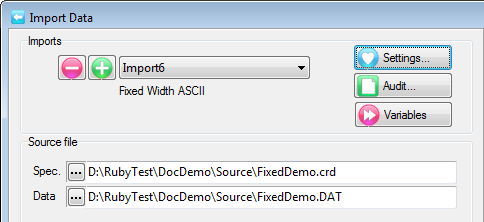
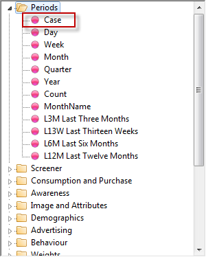
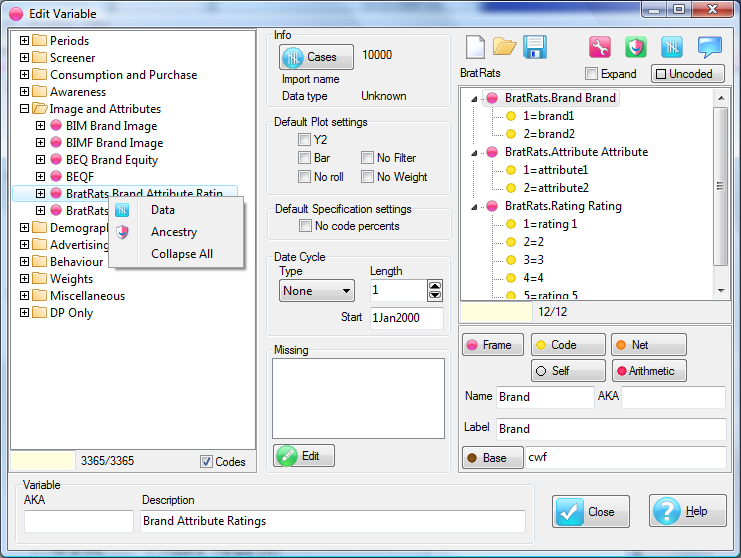
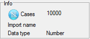
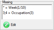
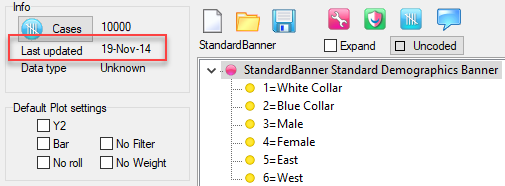
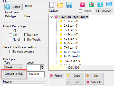
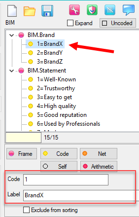
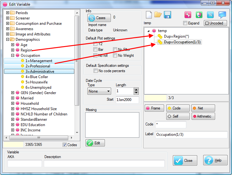
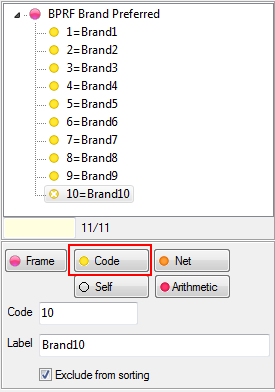
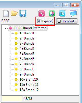
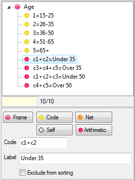
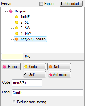
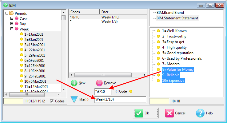
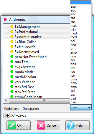
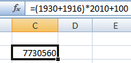
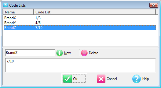
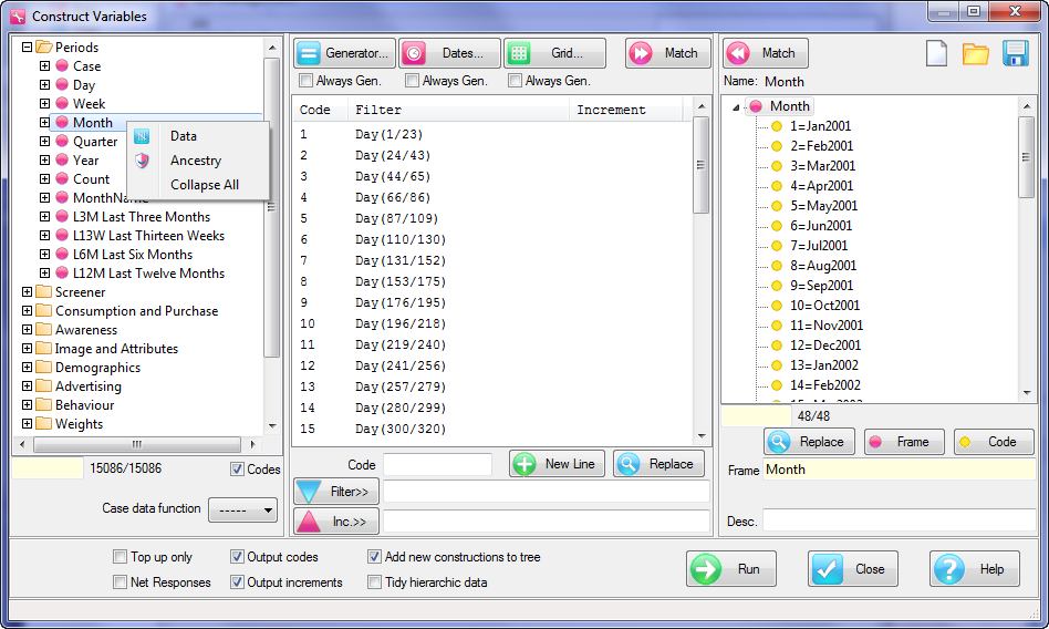
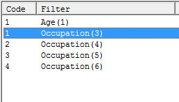
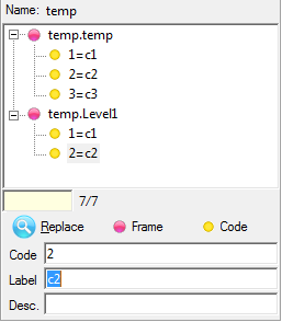

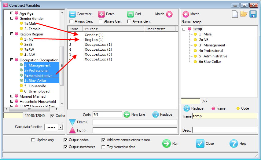
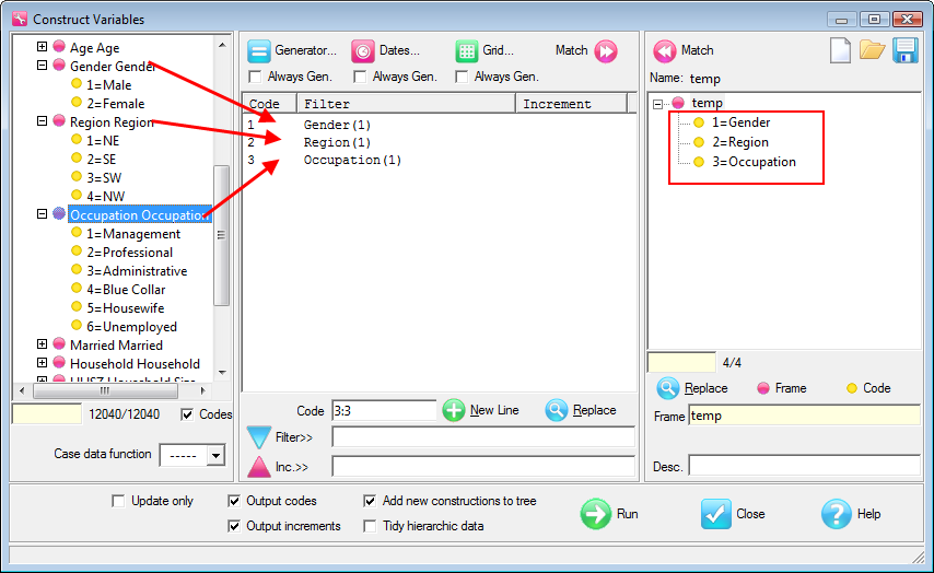
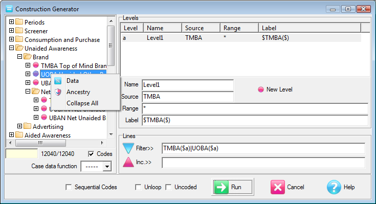
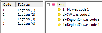
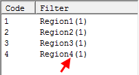
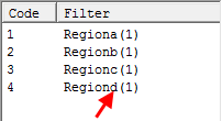
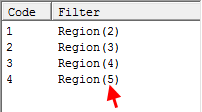
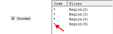
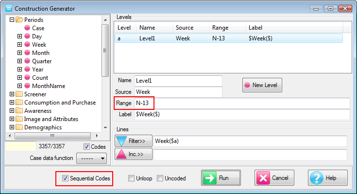
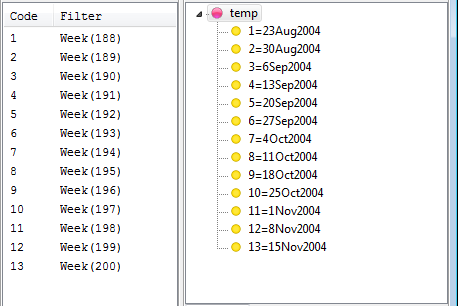
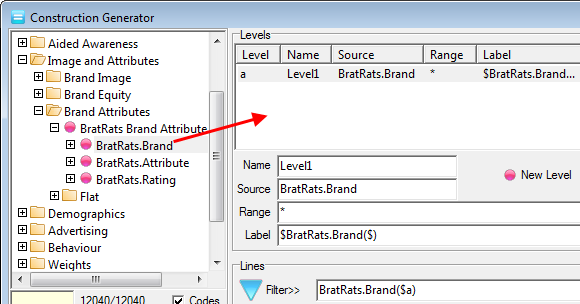
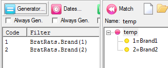
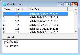
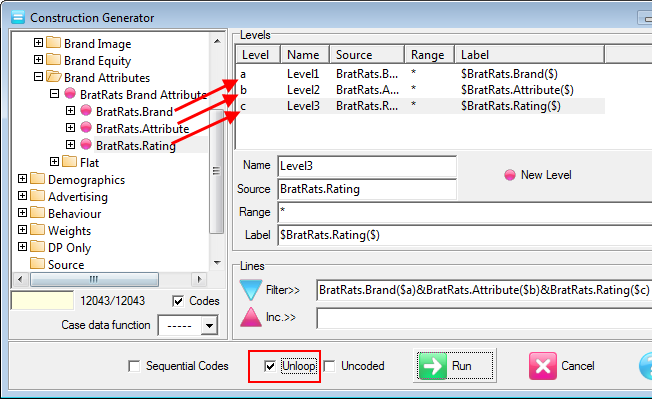
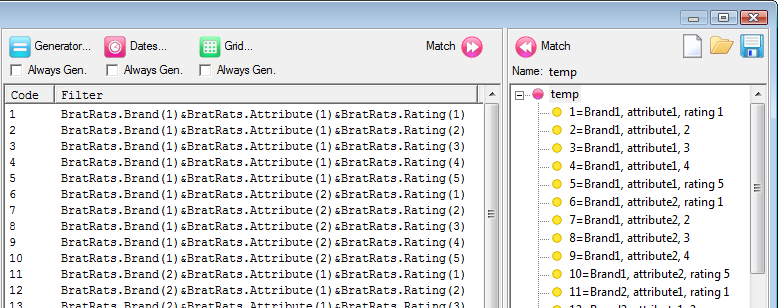
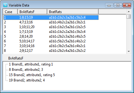
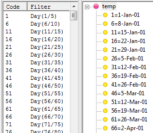
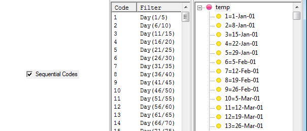
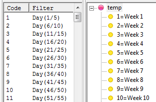
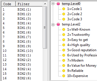
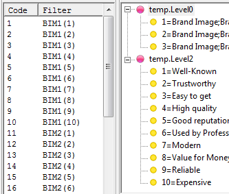
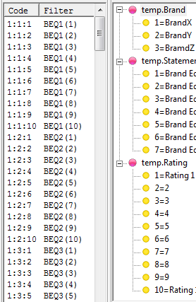
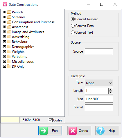
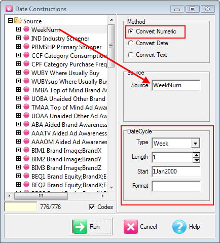
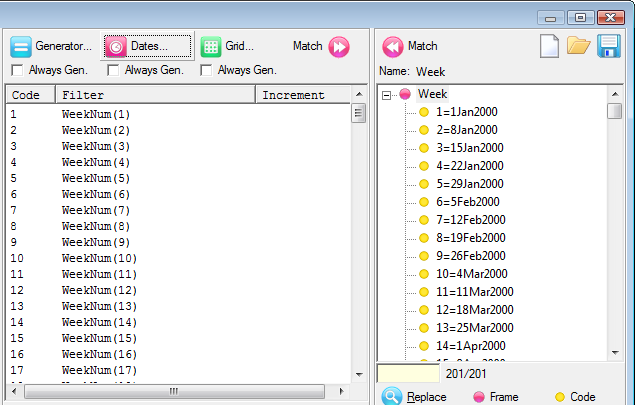
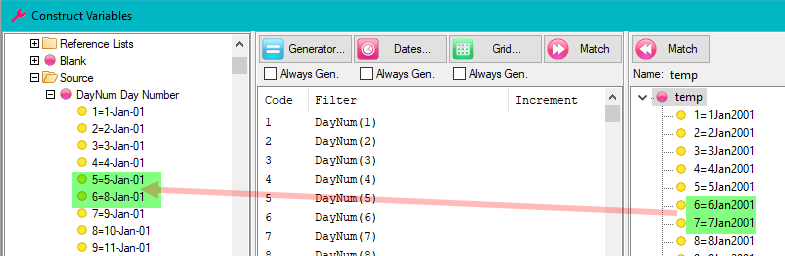
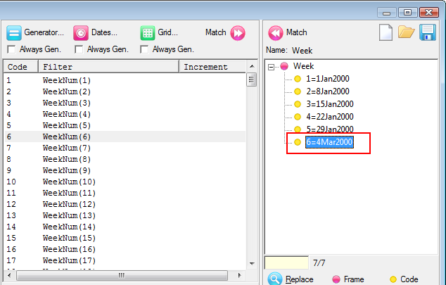
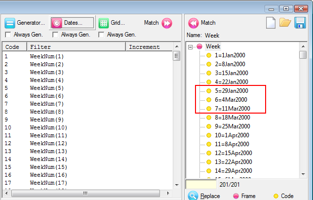
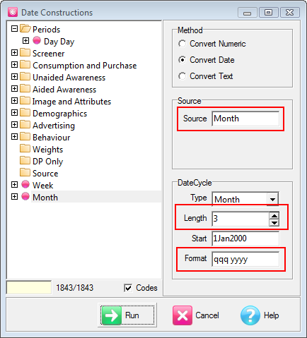
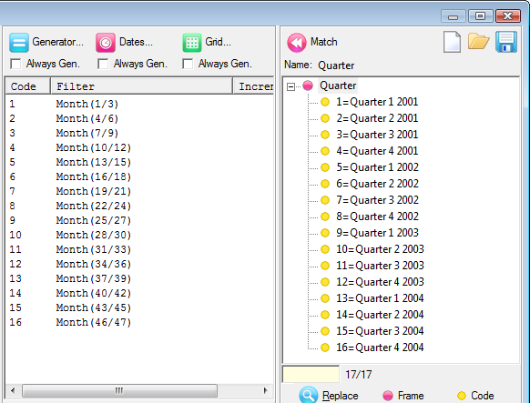
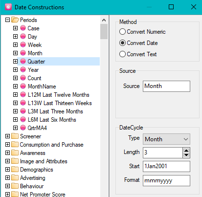
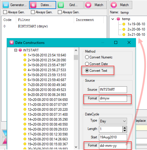
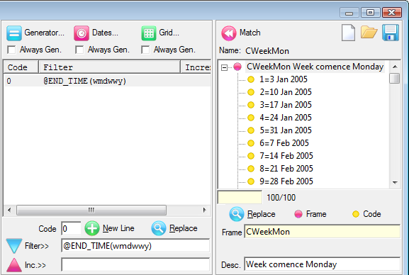
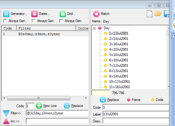
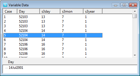
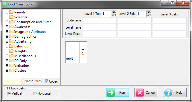
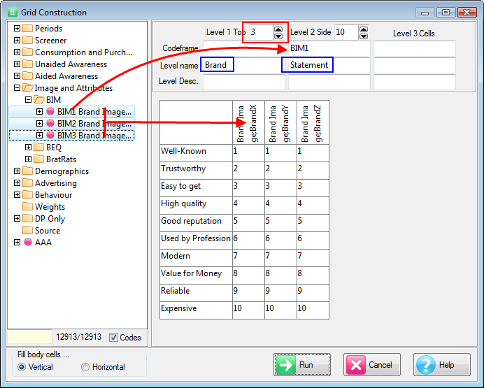
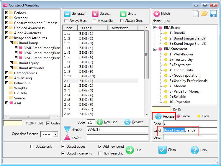
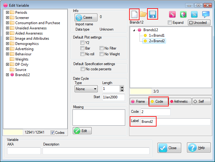
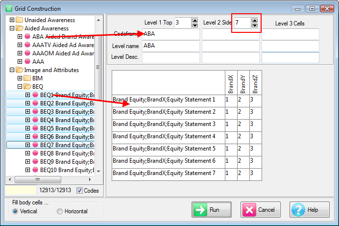
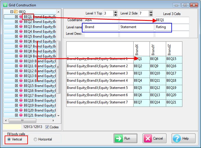
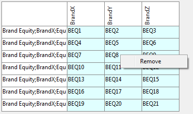
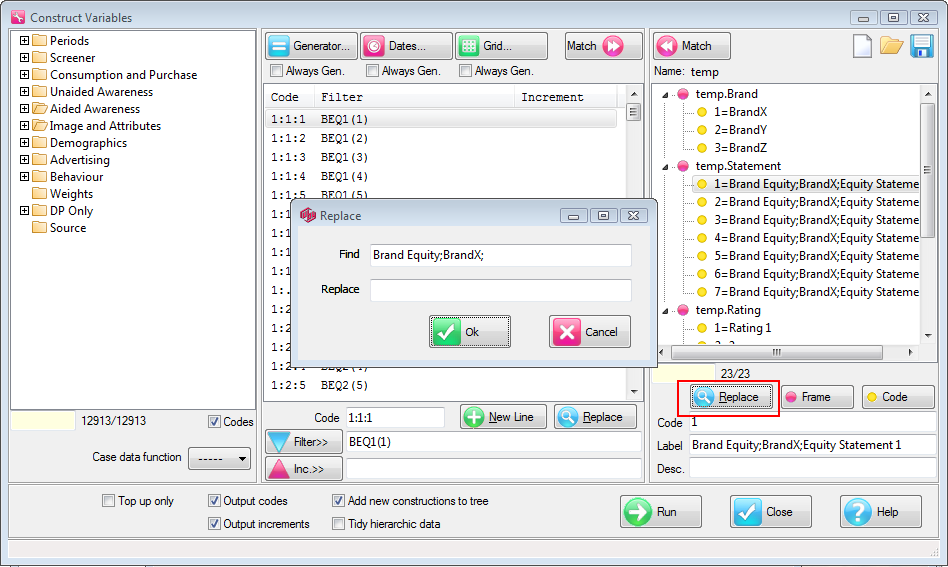
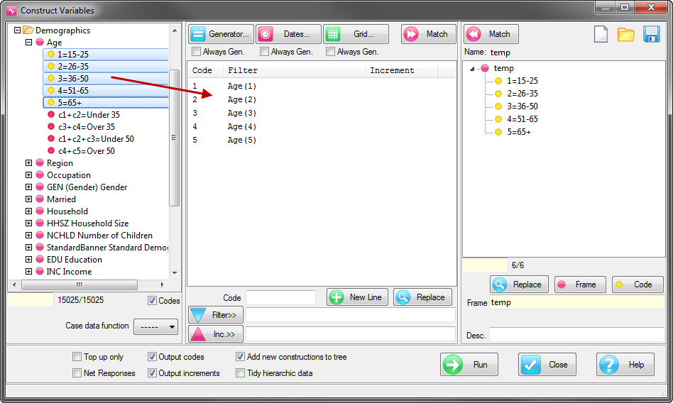
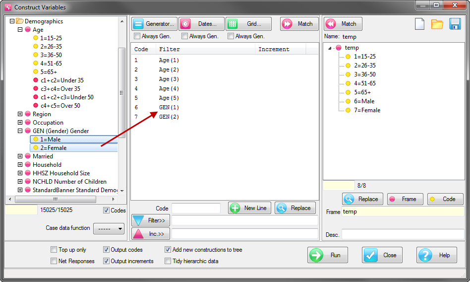
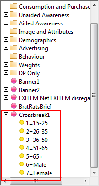

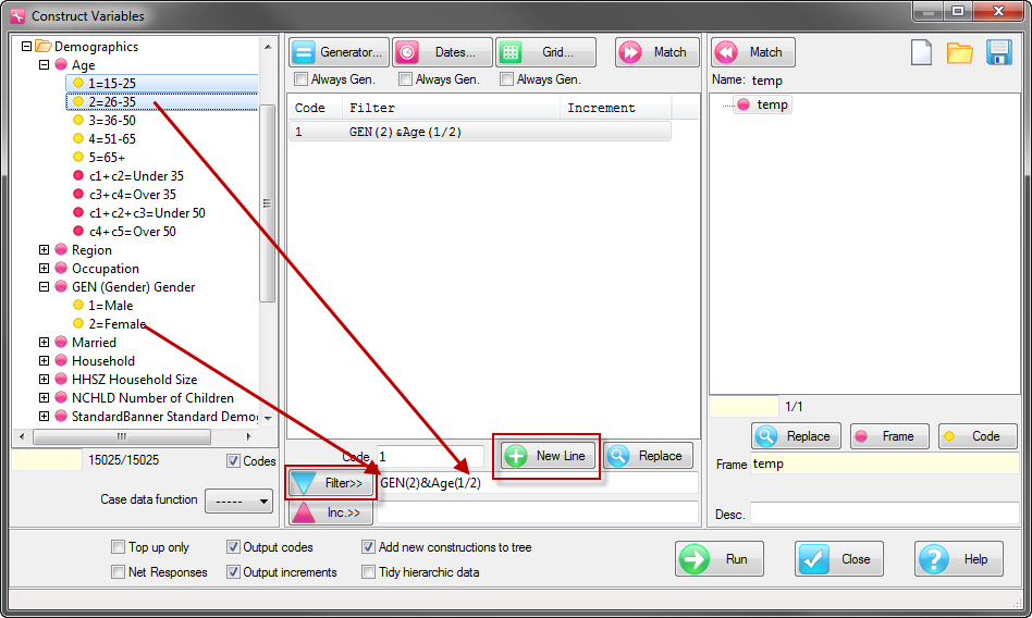
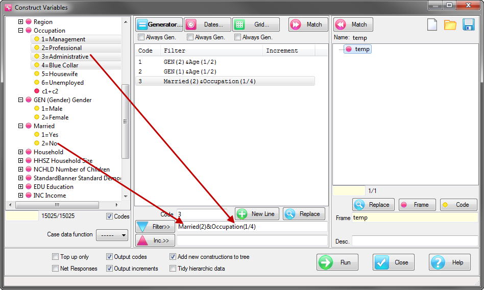
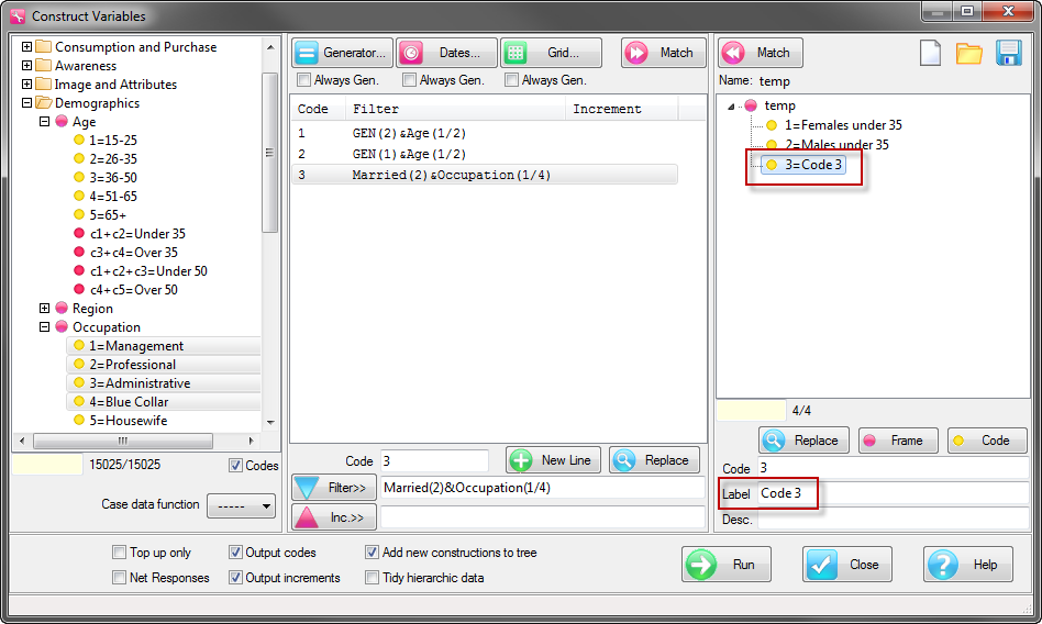
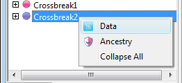
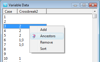
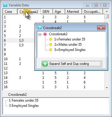
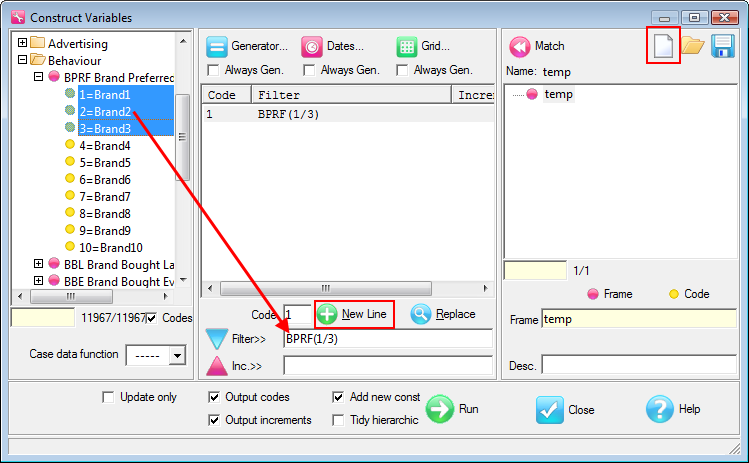
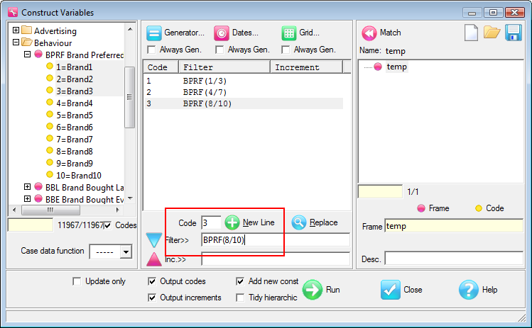
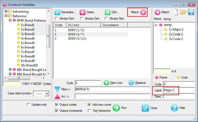
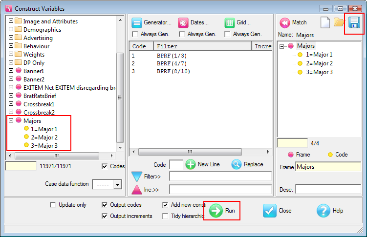
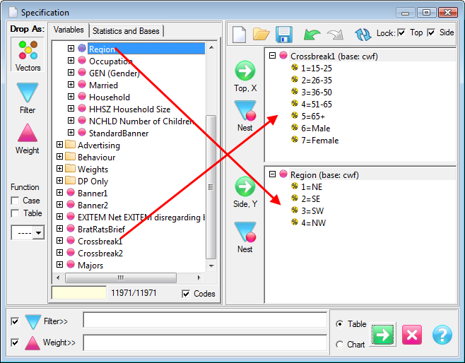
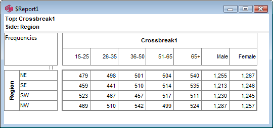
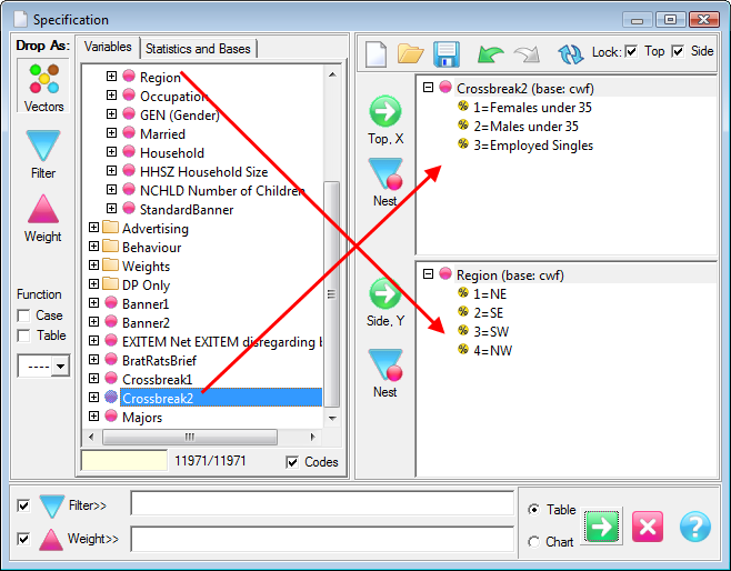
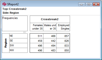

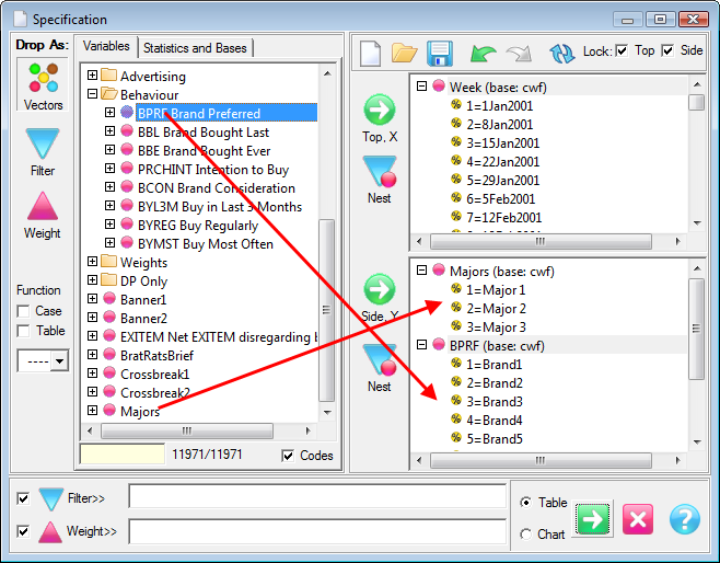
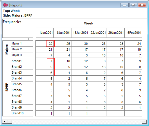
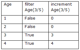
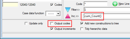
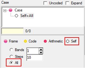
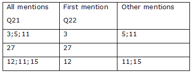
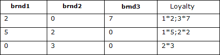
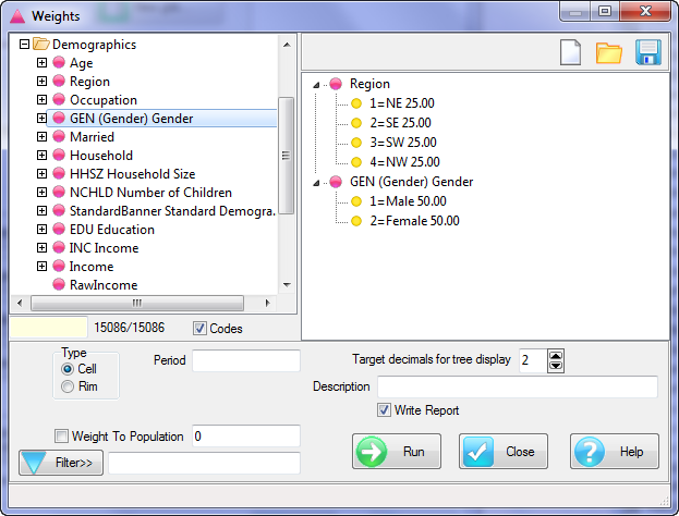
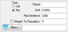
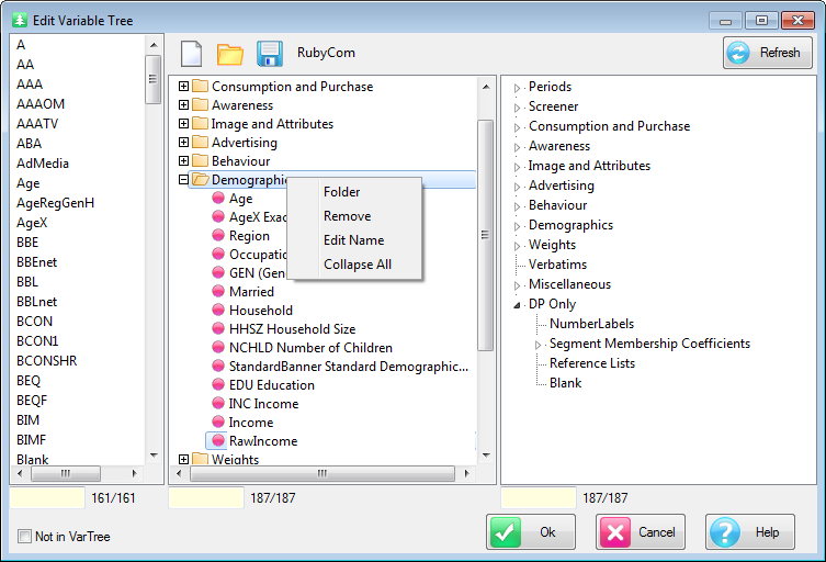
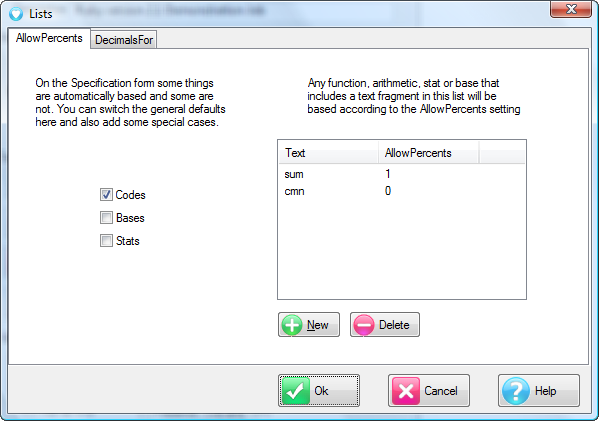
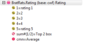
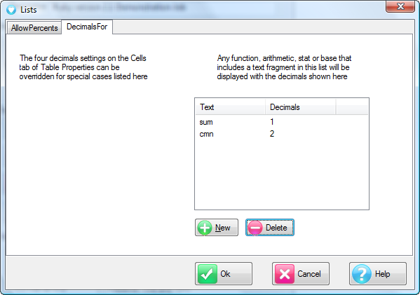
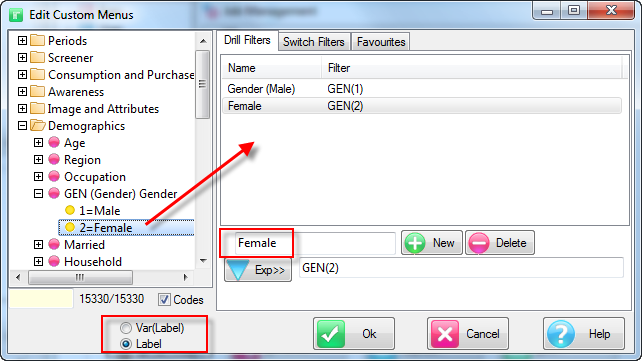
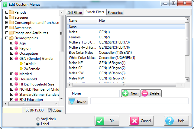
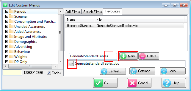
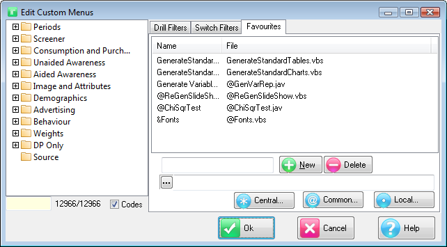

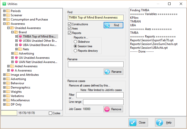

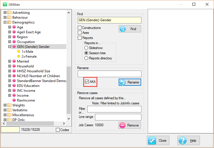
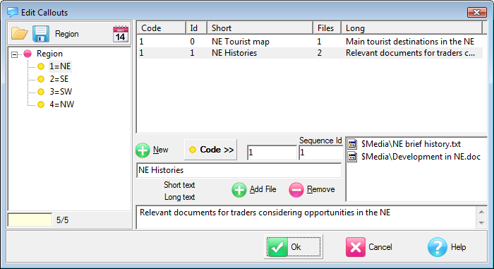
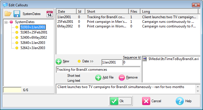
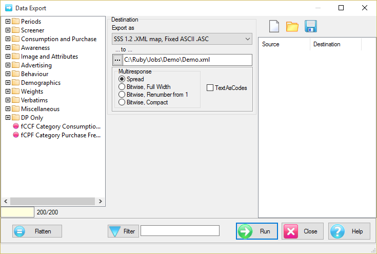

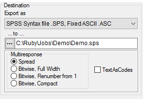
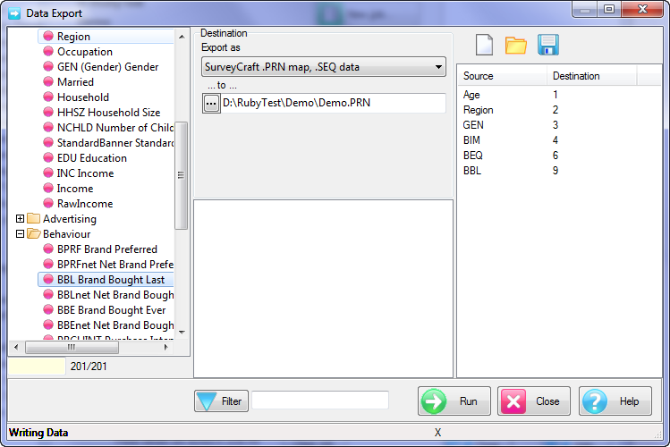
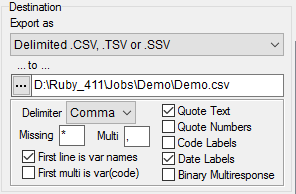
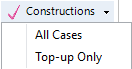
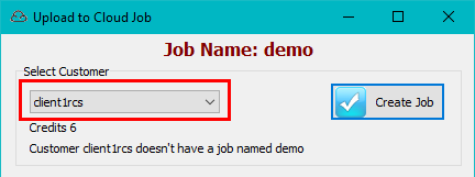
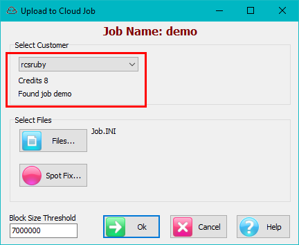
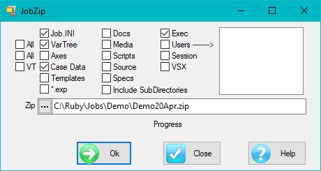
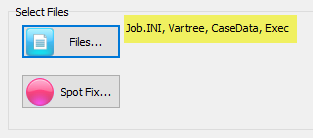
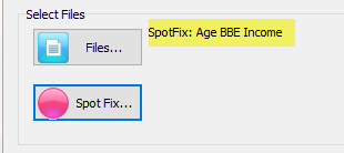
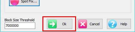
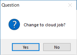
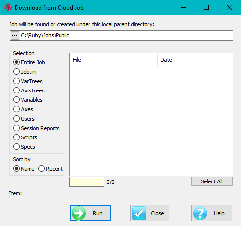
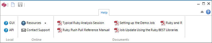

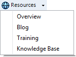
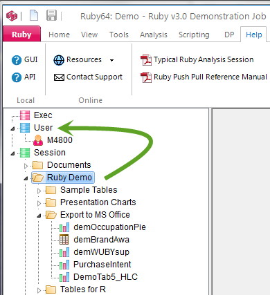
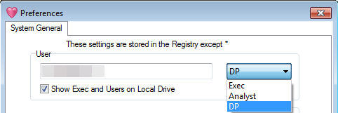
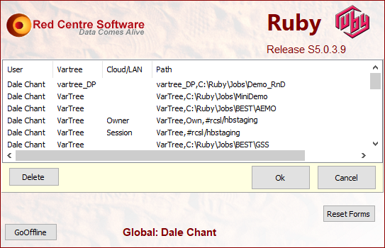
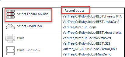
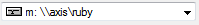
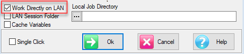
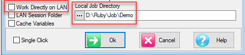
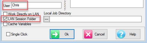
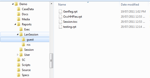
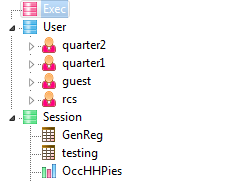
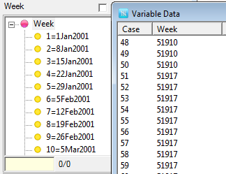
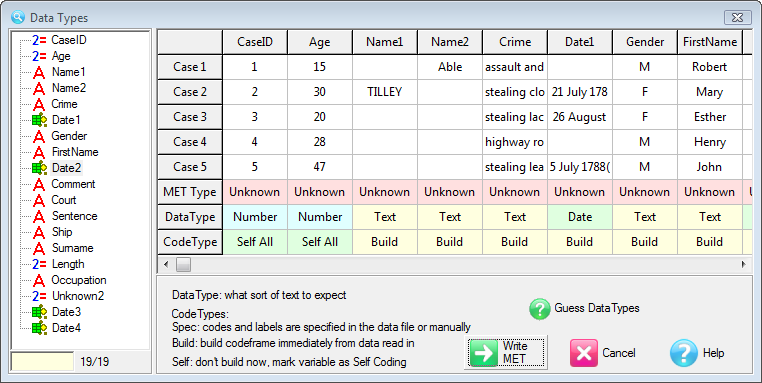
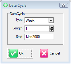
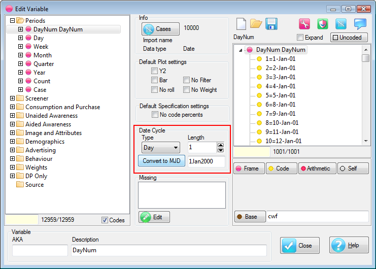
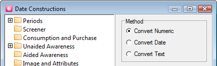
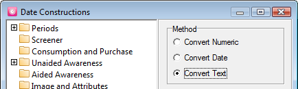
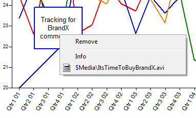
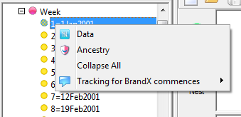
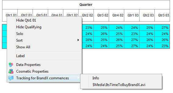
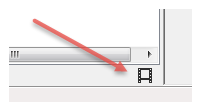
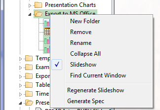
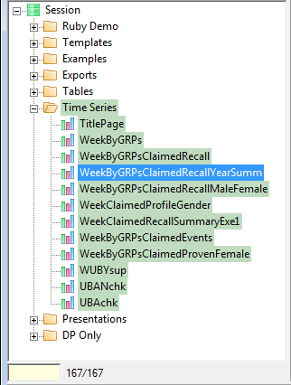
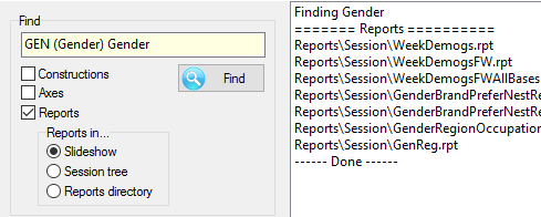
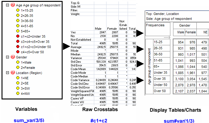
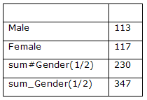
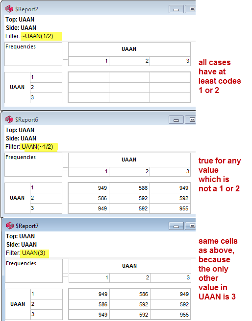
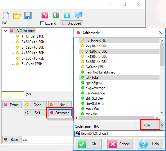
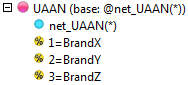
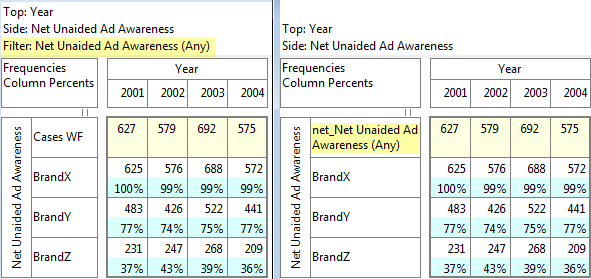
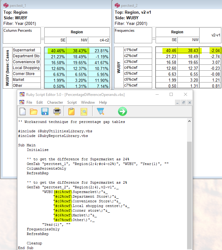
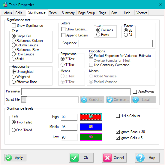
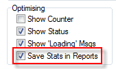
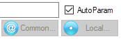
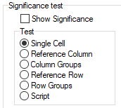
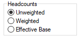
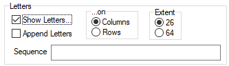
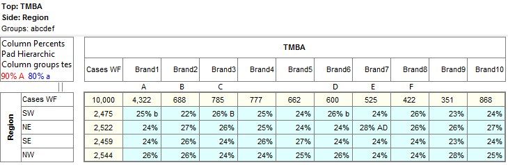
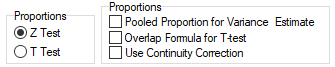
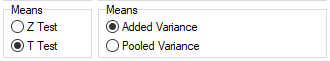

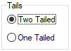
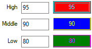
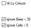
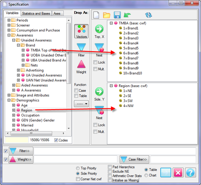
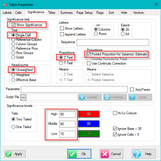
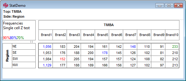
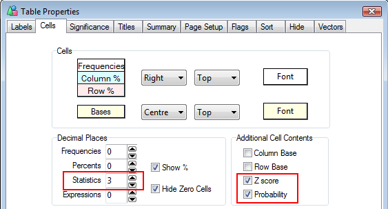
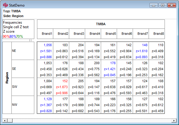
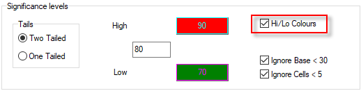
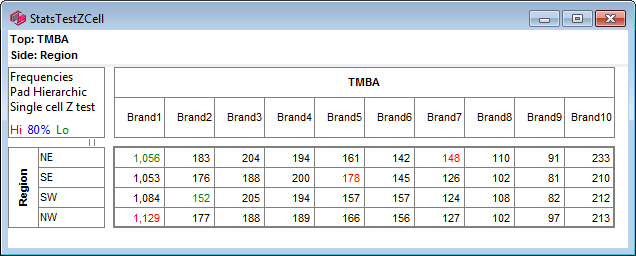
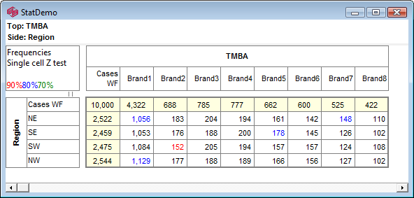
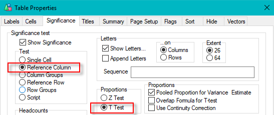
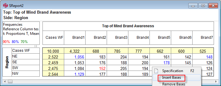
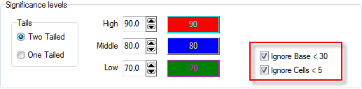
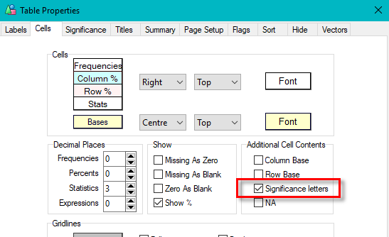
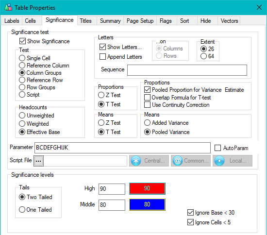
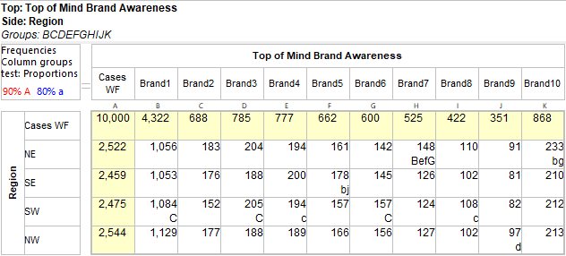
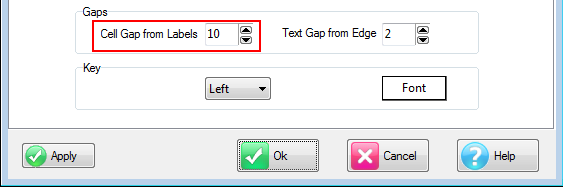
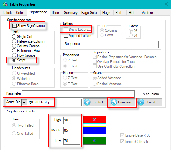
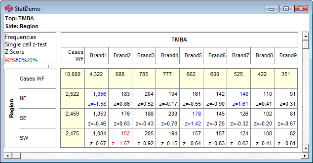
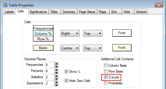
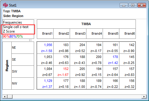
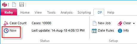
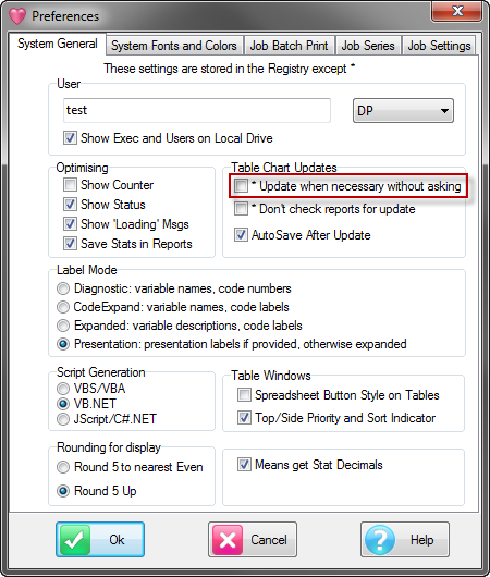
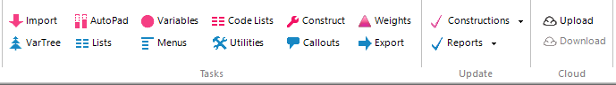
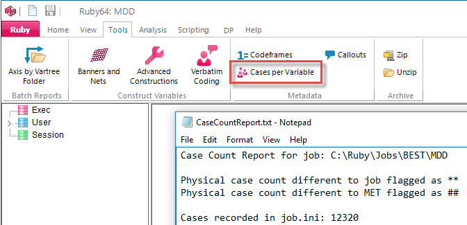

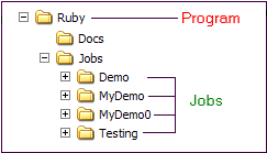
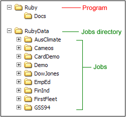
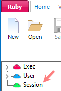
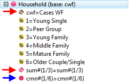
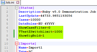
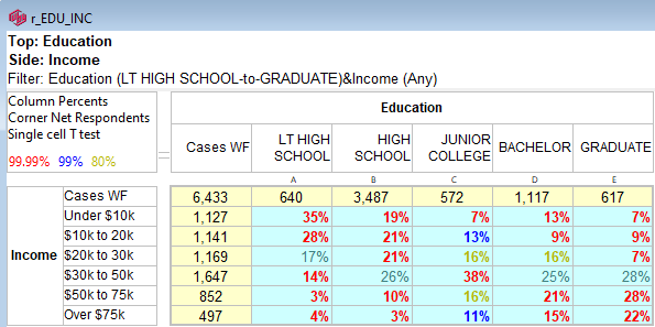
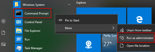
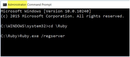
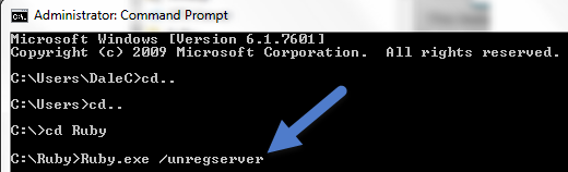
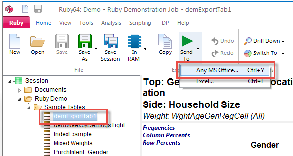
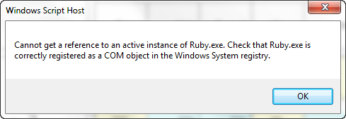
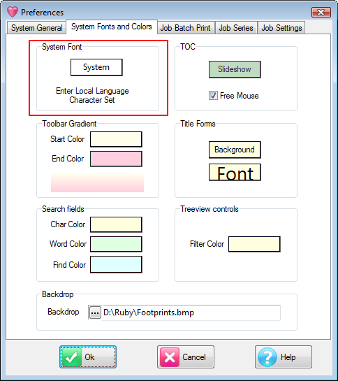
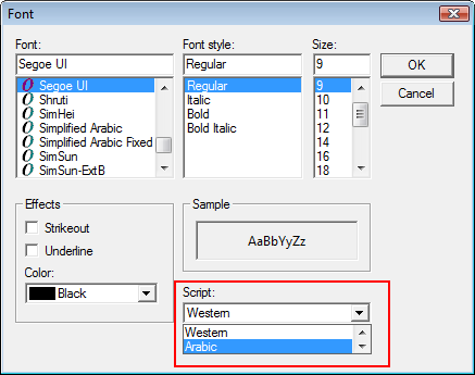
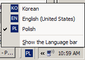
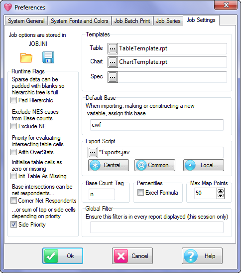
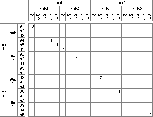
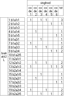
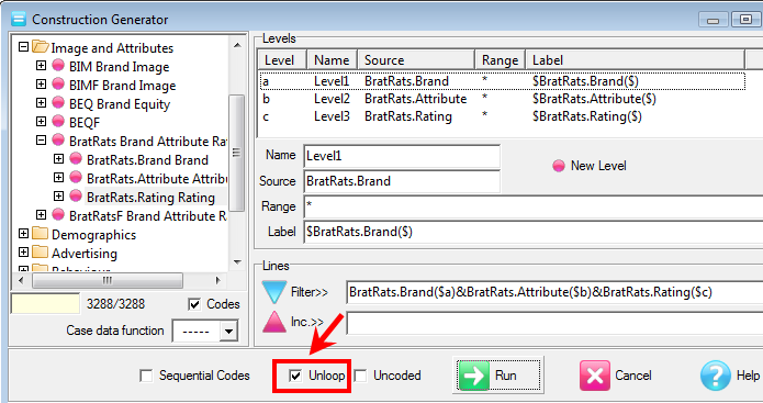
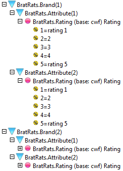
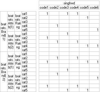
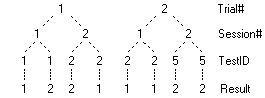
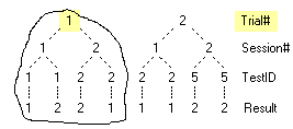
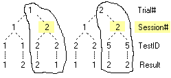
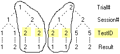
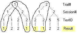
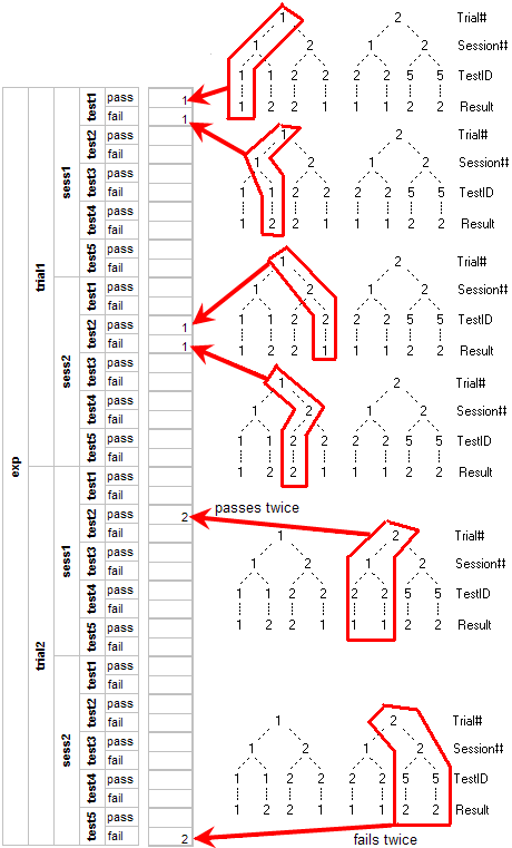
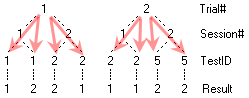
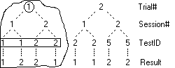
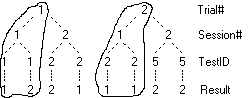
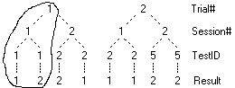
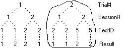
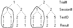
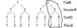
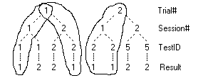
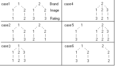
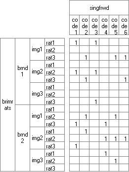
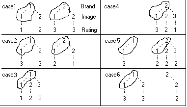
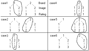
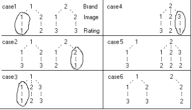
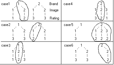
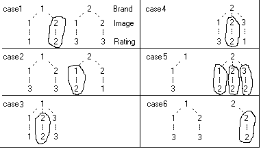
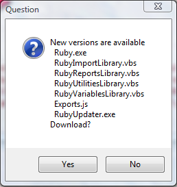

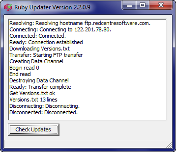
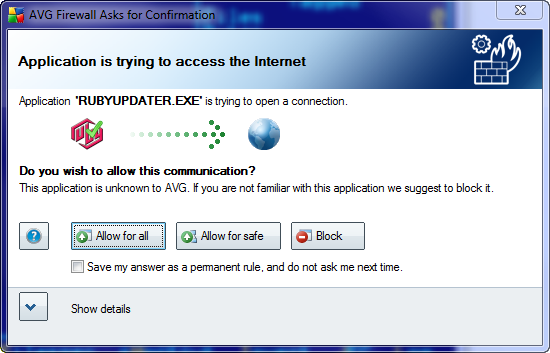
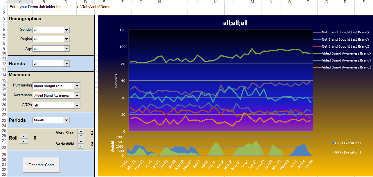
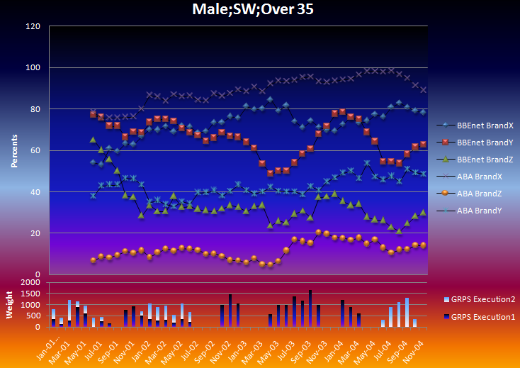
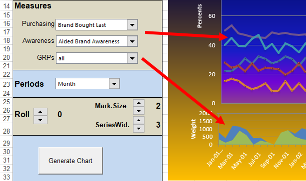
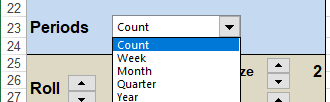
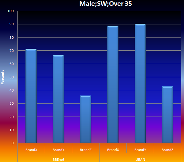
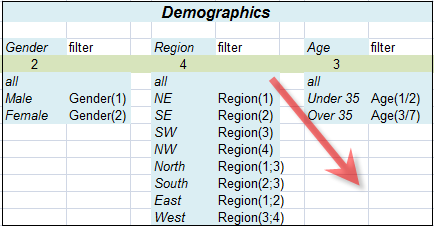
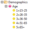
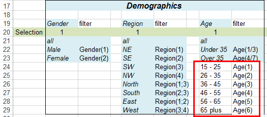
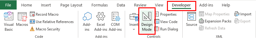
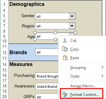
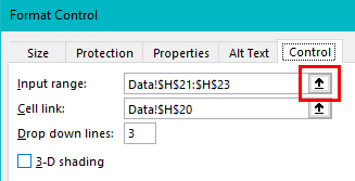
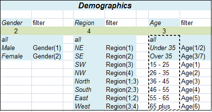
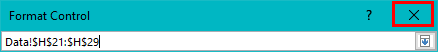
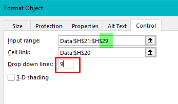
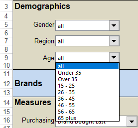
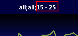
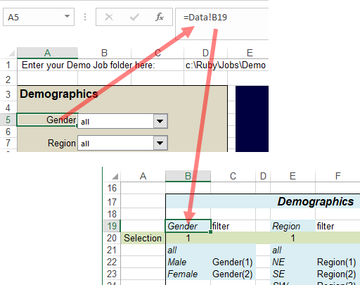
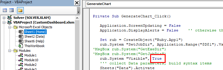
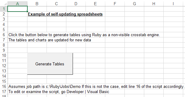
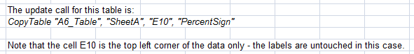
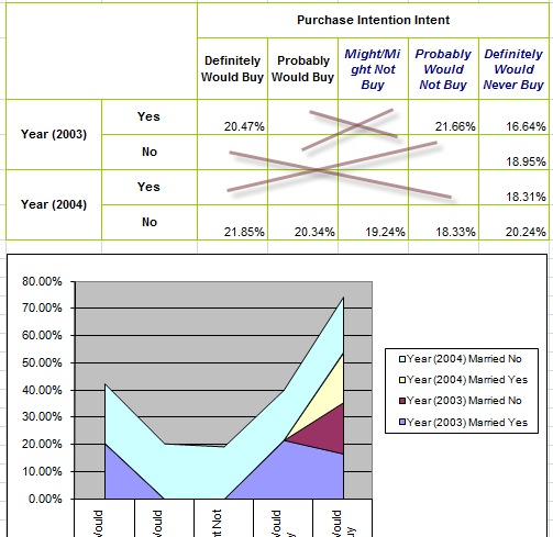
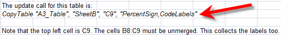
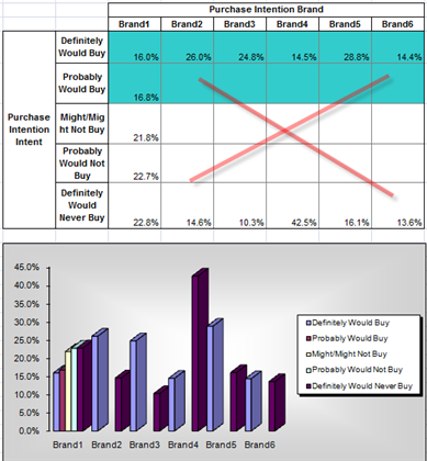
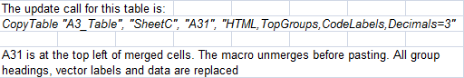
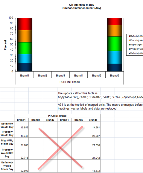
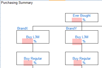
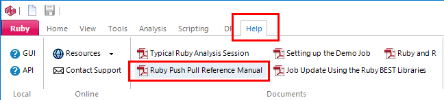
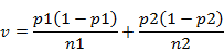
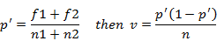
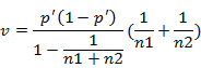
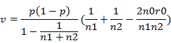
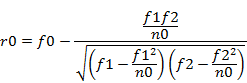
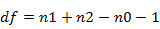
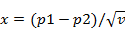
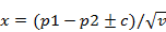
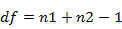
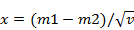

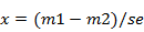
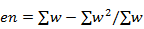
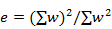
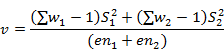
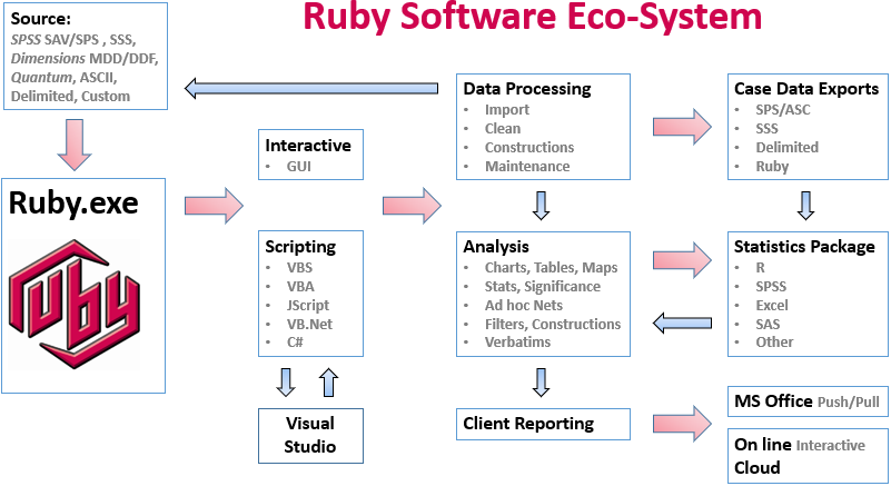
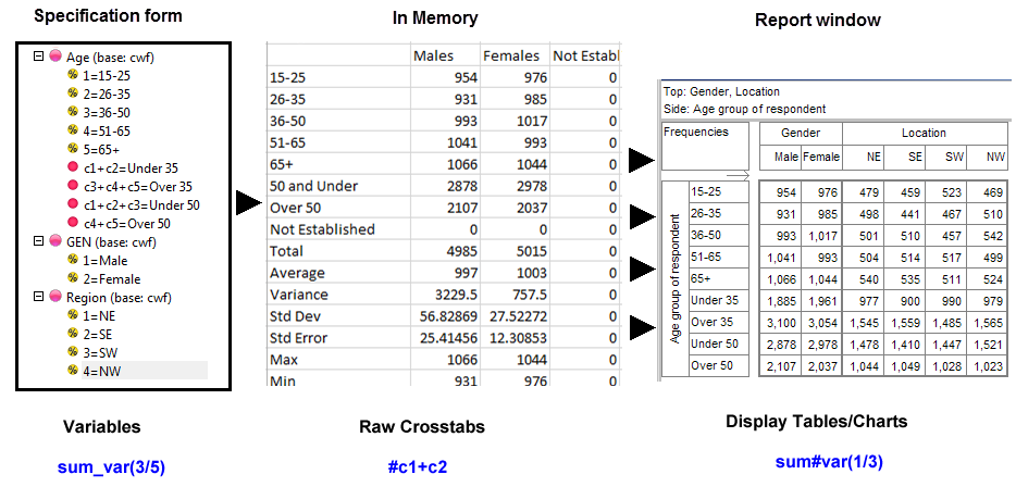
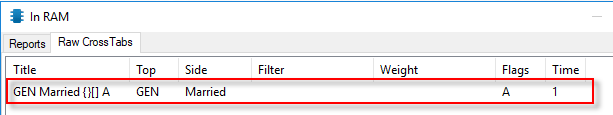
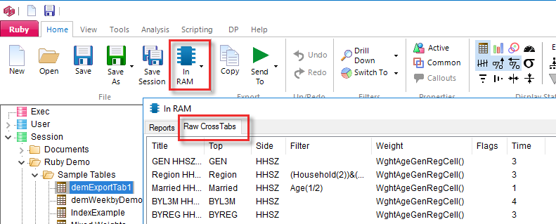
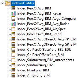
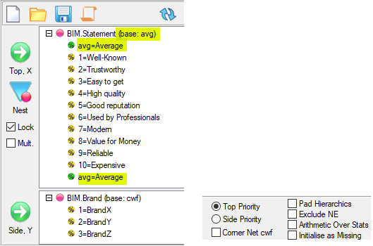
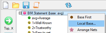
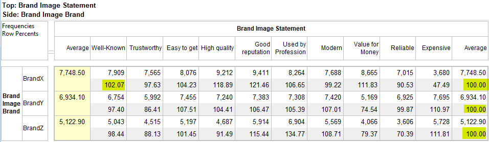
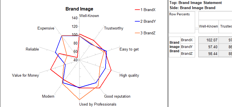
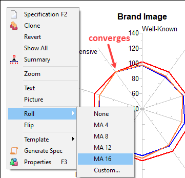
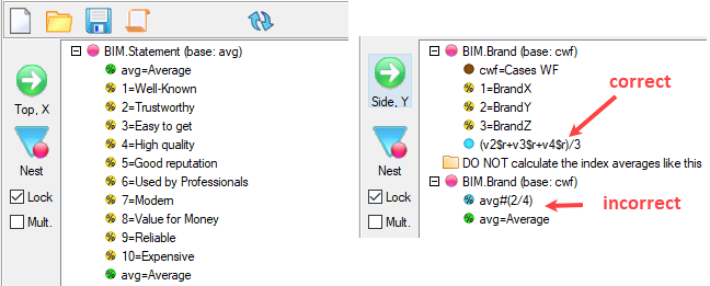
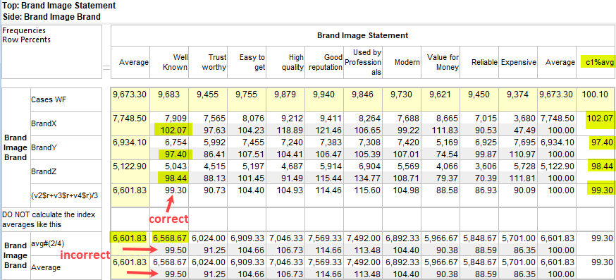
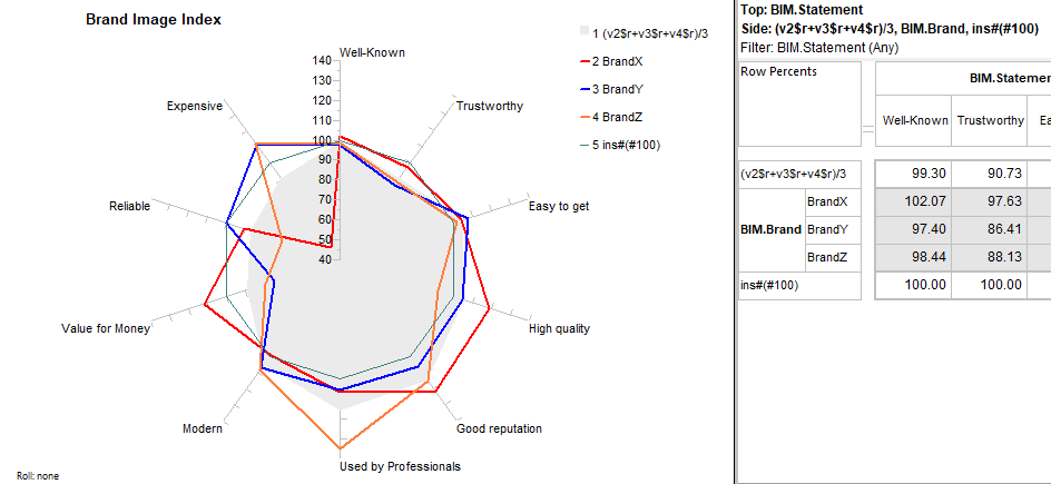
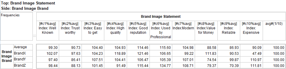
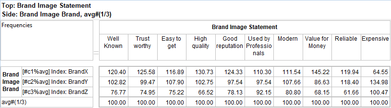
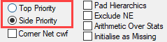
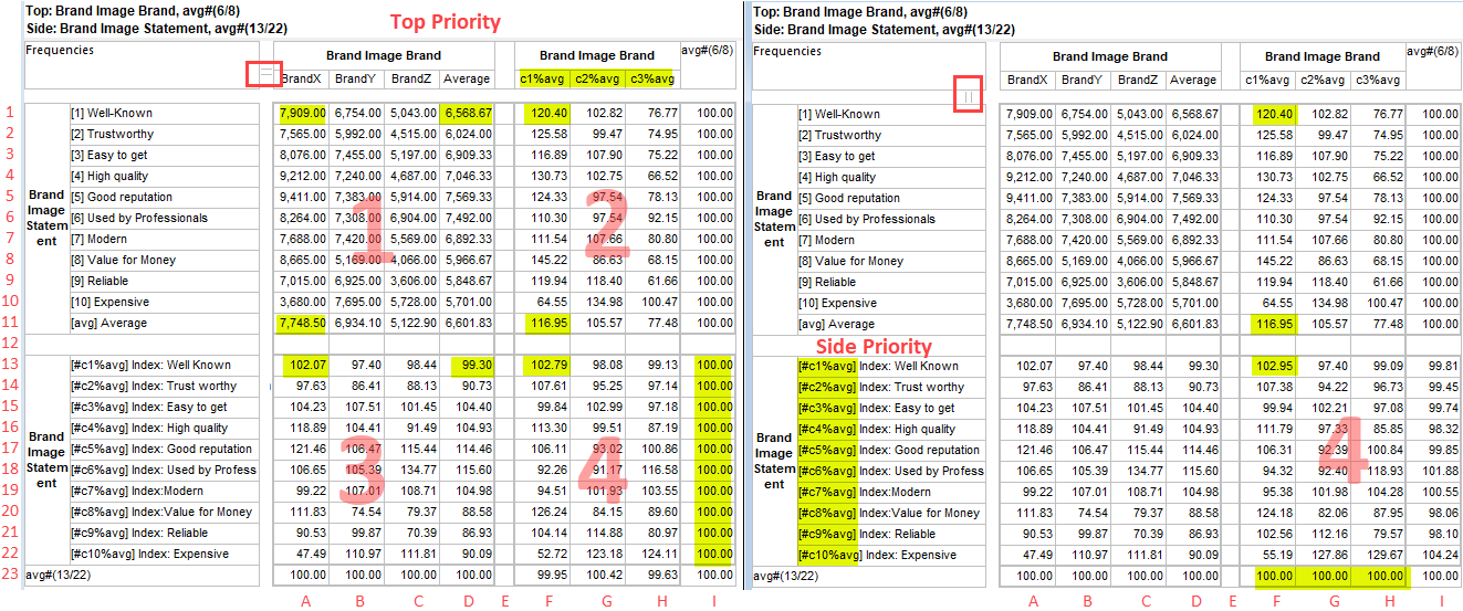
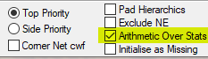
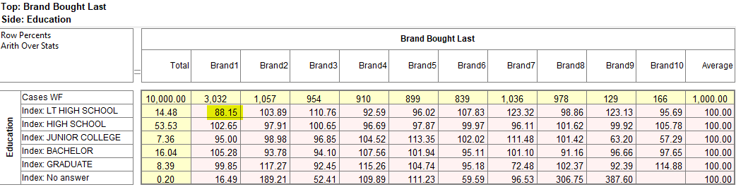
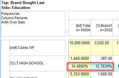
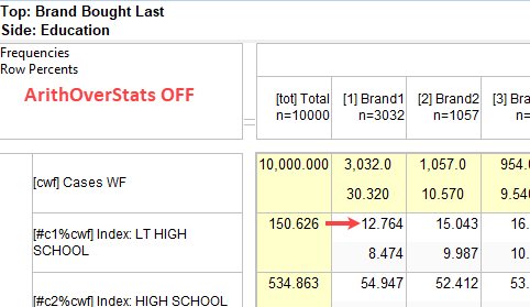
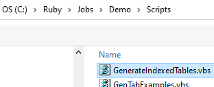
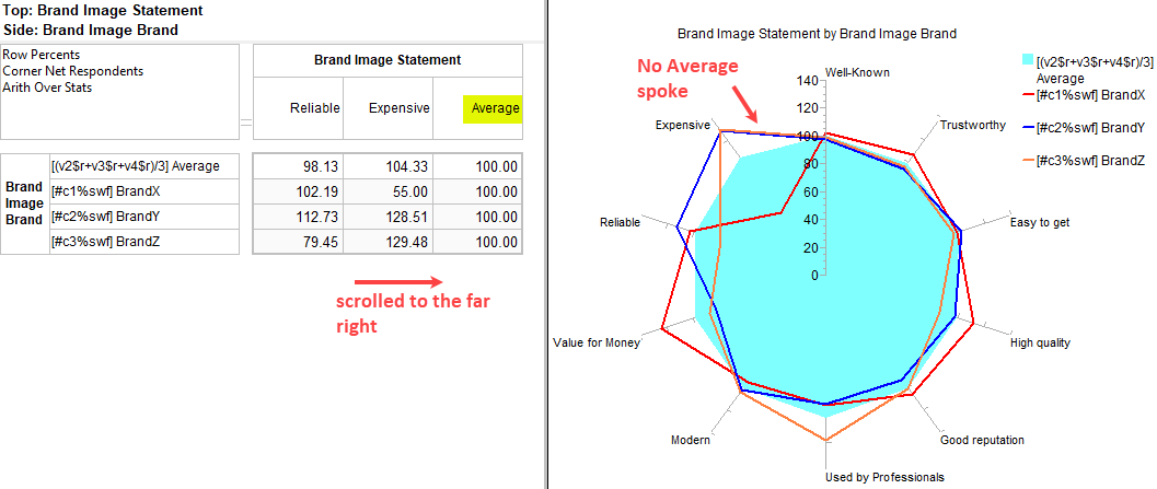
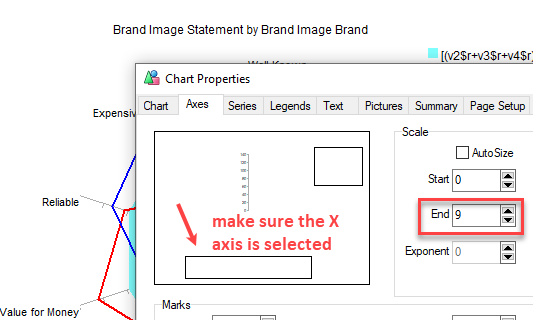
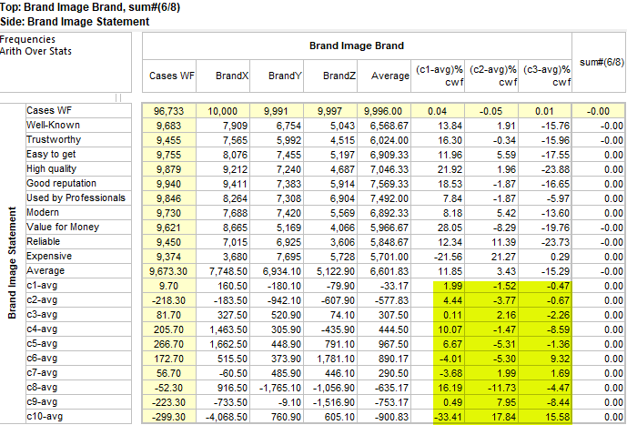
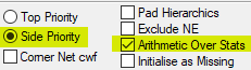
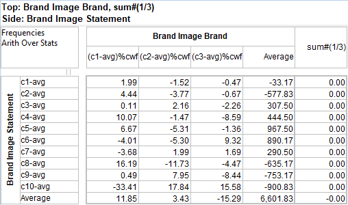
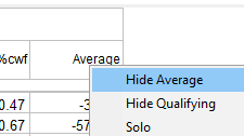
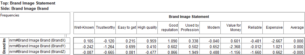
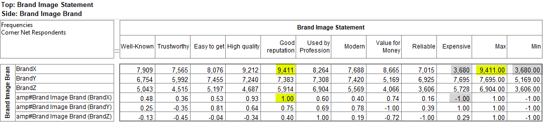
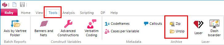

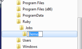
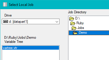
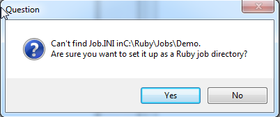
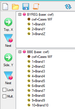
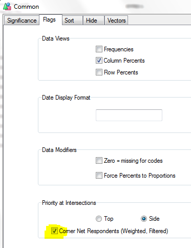
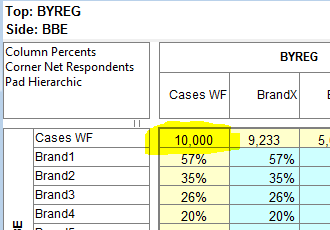
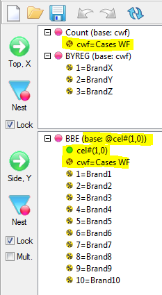
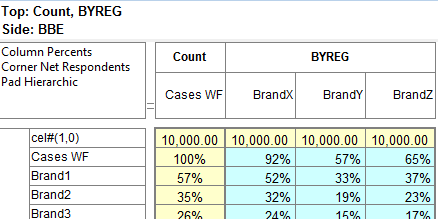
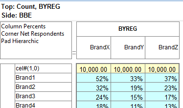
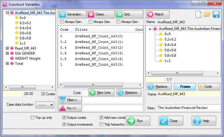
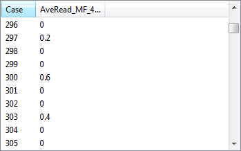
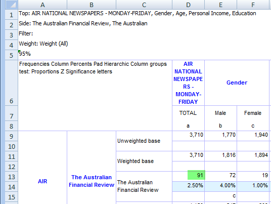
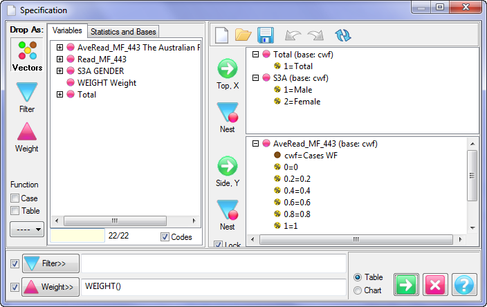
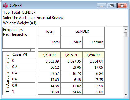
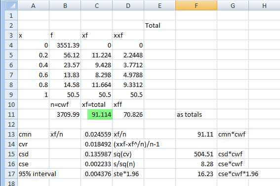


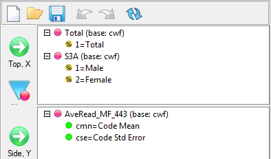
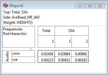
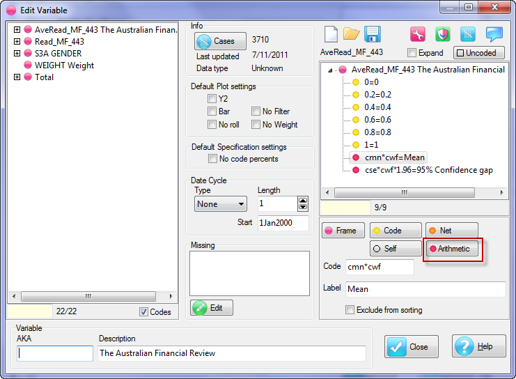
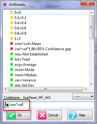
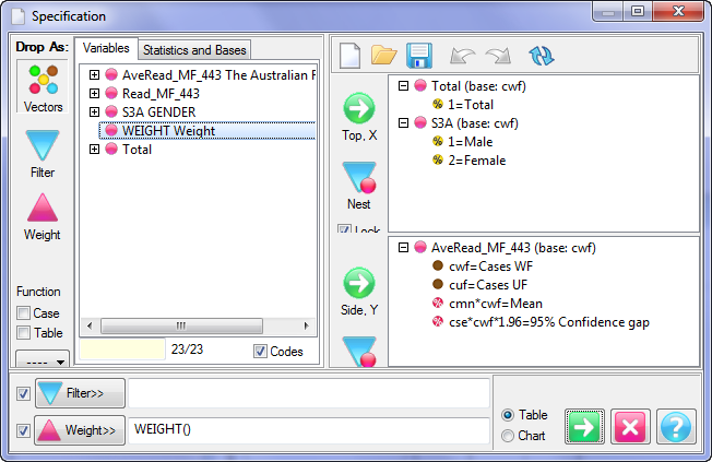
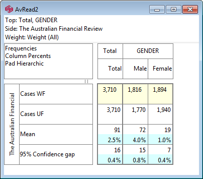
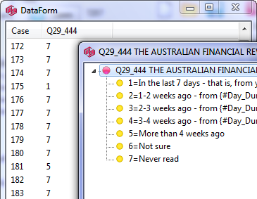
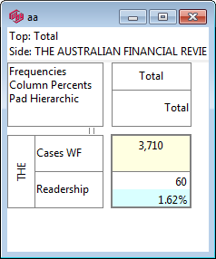
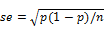
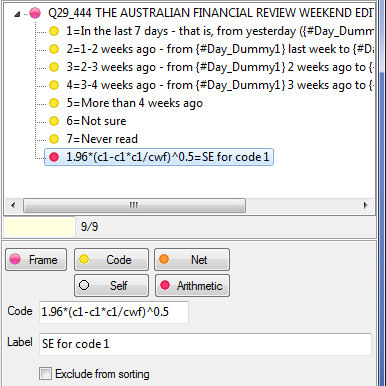
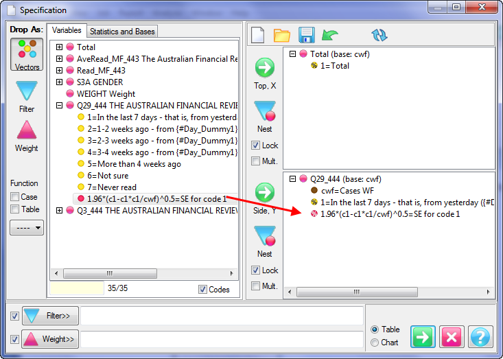
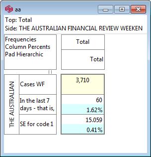
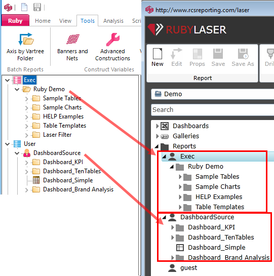
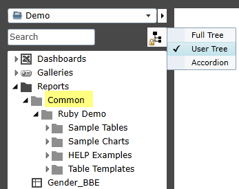
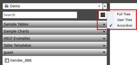
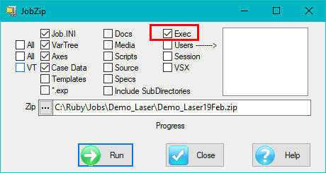
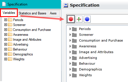
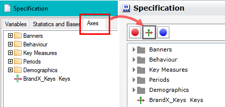
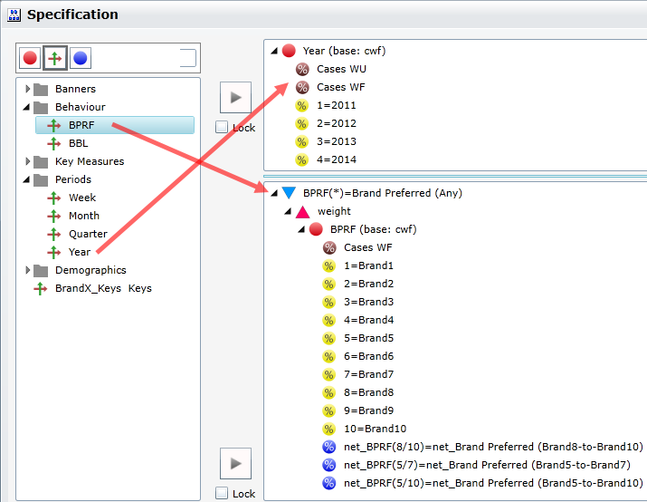
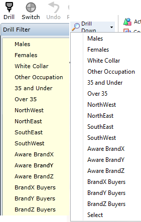
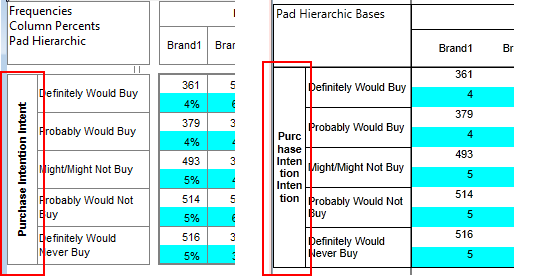
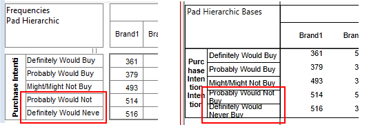
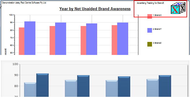
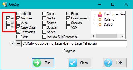
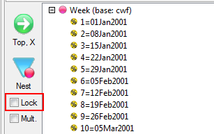
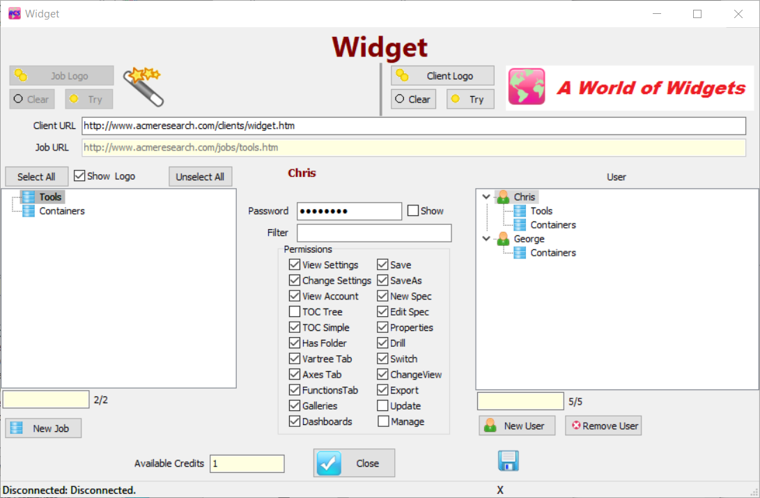
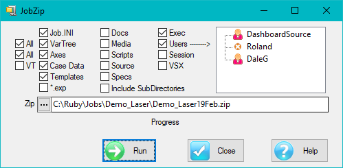
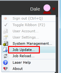
Was this article helpful?
That’s Great!
Thank you for your feedback
Sorry! We couldn't be helpful
Thank you for your feedback
Feedback sent
We appreciate your effort and will try to fix the article